7 Kanku-Breakaways
7.1 Continuous
7.1.1 elev
Figure 7.1 shows rasters for elev in the Kanku-Breakaways area.
Table 7.2 shows boxplots for each decile of elev, allowing a comparison of values within each DEM across different ranges of elev. Deciles are based on the values in the reference DEM: Outback.
Figure 7.3 shows the a distribution of values for each sample DEM and window size.
Figure 7.4 shows the distribution of differences between the reference DEM and the other DEMs.
Figure 7.1: elev raster for each DEM
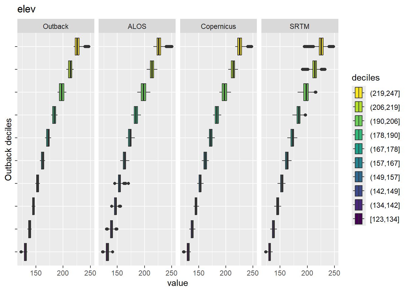
Figure 7.2: Range of values within deciles for each DEM. Deciles are taken from the reference DEM
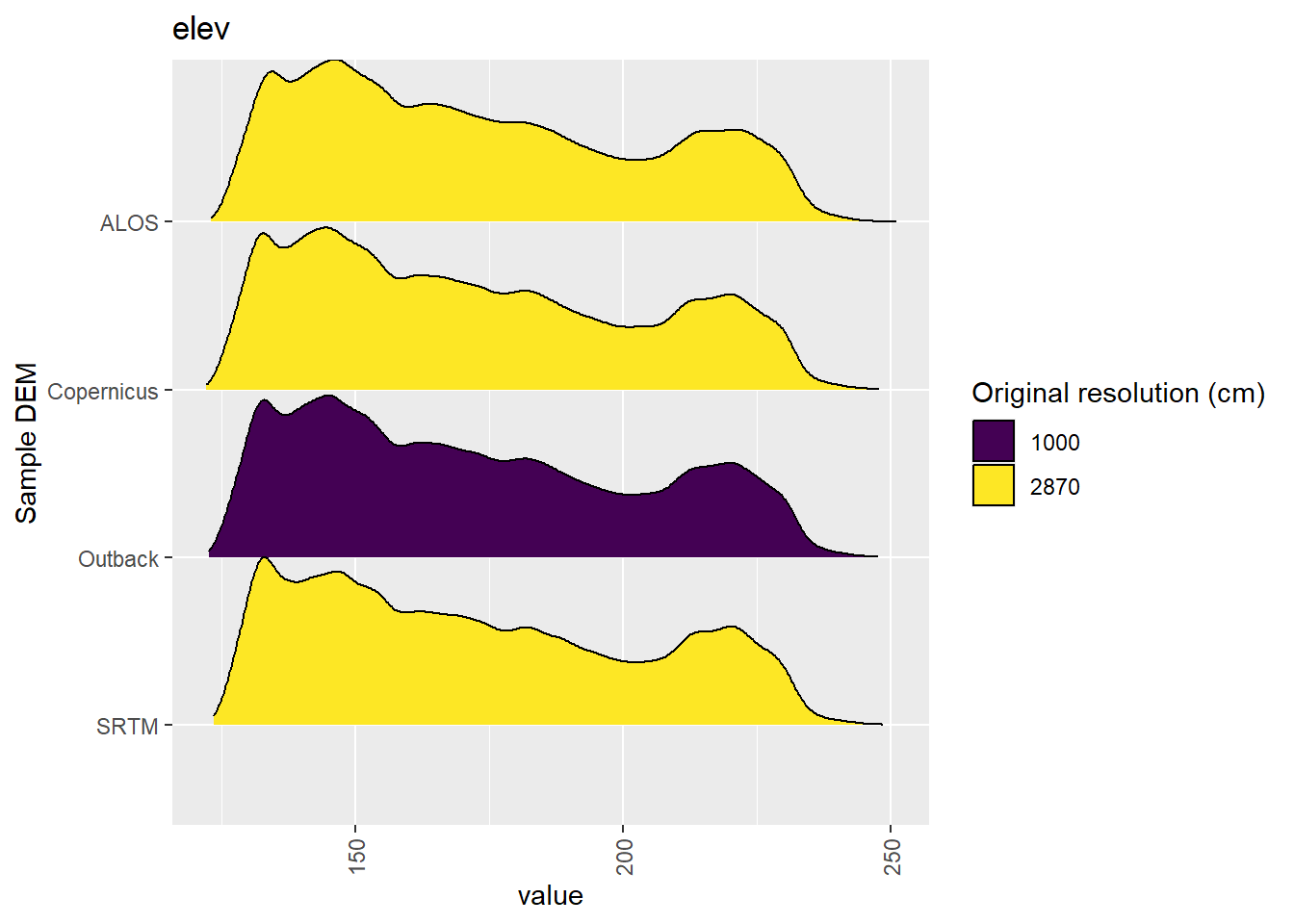
Figure 7.3: Distribution of elev values in each DEM: Kanku-Breakaways
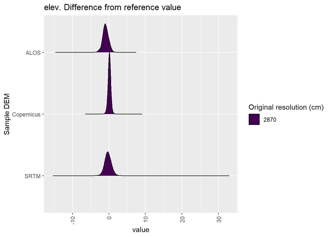
Figure 7.4: Distribution of difference between each DEM and reference for elev values: Kanku-Breakaways
7.1.2 qslope
Figure 7.5 shows rasters for qslope in the Kanku-Breakaways area.
Table 7.6 shows boxplots for each decile of qslope, allowing a comparison of values within each DEM across different ranges of qslope. Deciles are based on the values in the reference DEM: Outback.
Figure 7.7 shows the a distribution of values for each sample DEM and window size.
Figure 7.8 shows the distribution of differences between the reference DEM and the other DEMs.
Figure 7.5: qslope raster for each DEM
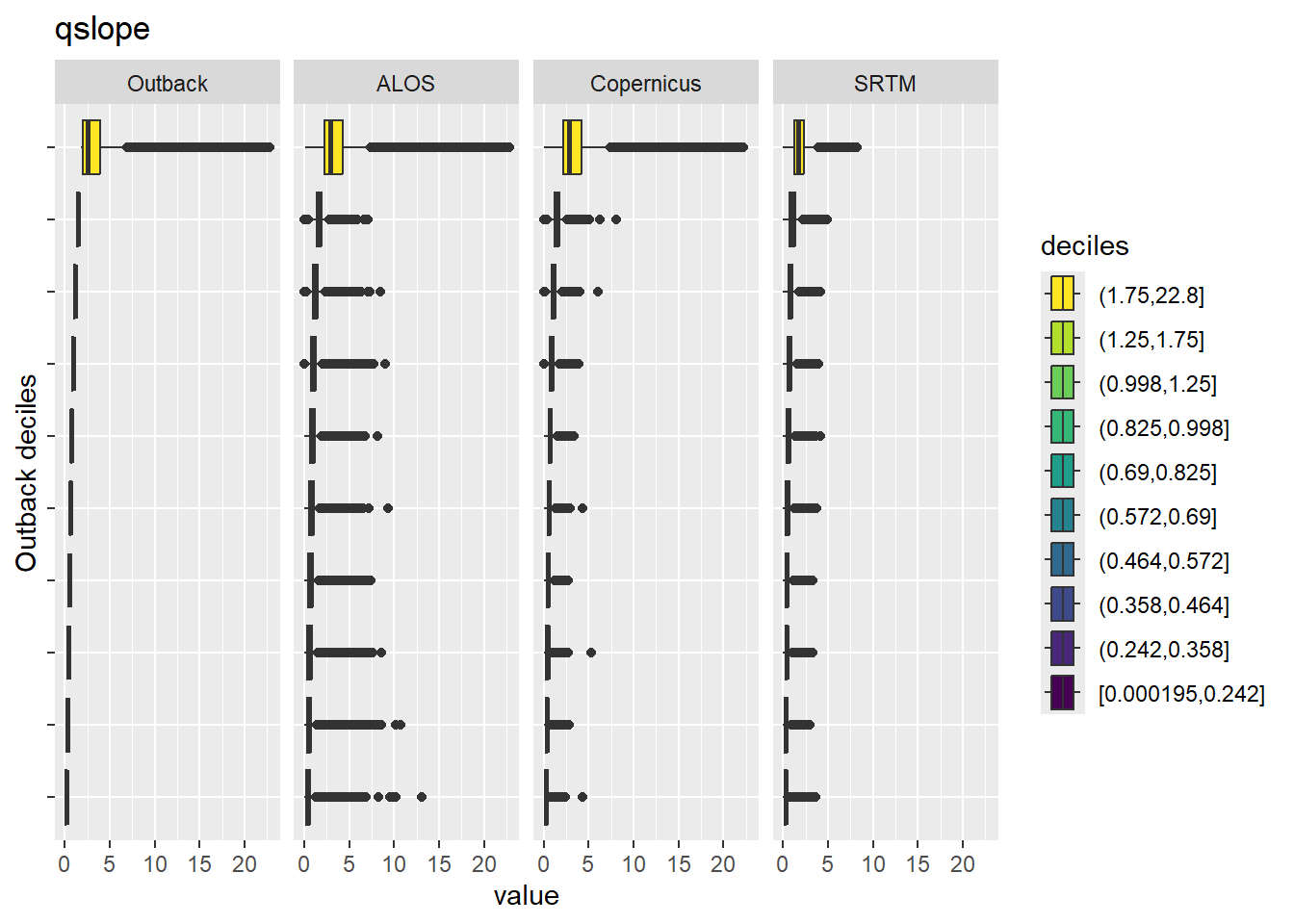
Figure 7.6: Range of values within deciles for each DEM. Deciles are taken from the reference DEM
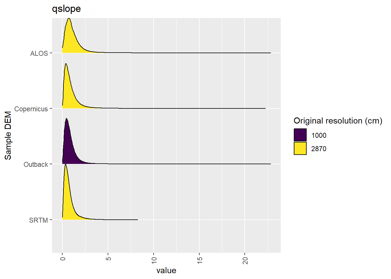
Figure 7.7: Distribution of qslope values in each DEM: Kanku-Breakaways
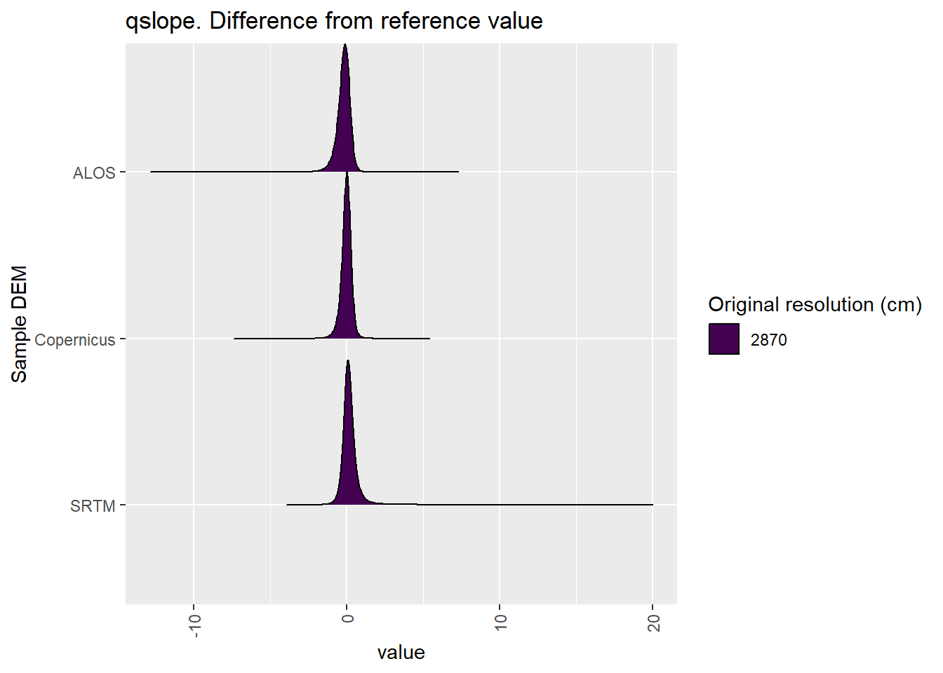
Figure 7.8: Distribution of difference between each DEM and reference for qslope values: Kanku-Breakaways
7.1.3 qaspect
Figure 7.9 shows rasters for qaspect in the Kanku-Breakaways area.
Table 7.10 shows boxplots for each decile of qaspect, allowing a comparison of values within each DEM across different ranges of qaspect. Deciles are based on the values in the reference DEM: Outback.
Figure 7.11 shows the a distribution of values for each sample DEM and window size.
Figure 7.12 shows the distribution of differences between the reference DEM and the other DEMs.
Figure 7.9: qaspect raster for each DEM
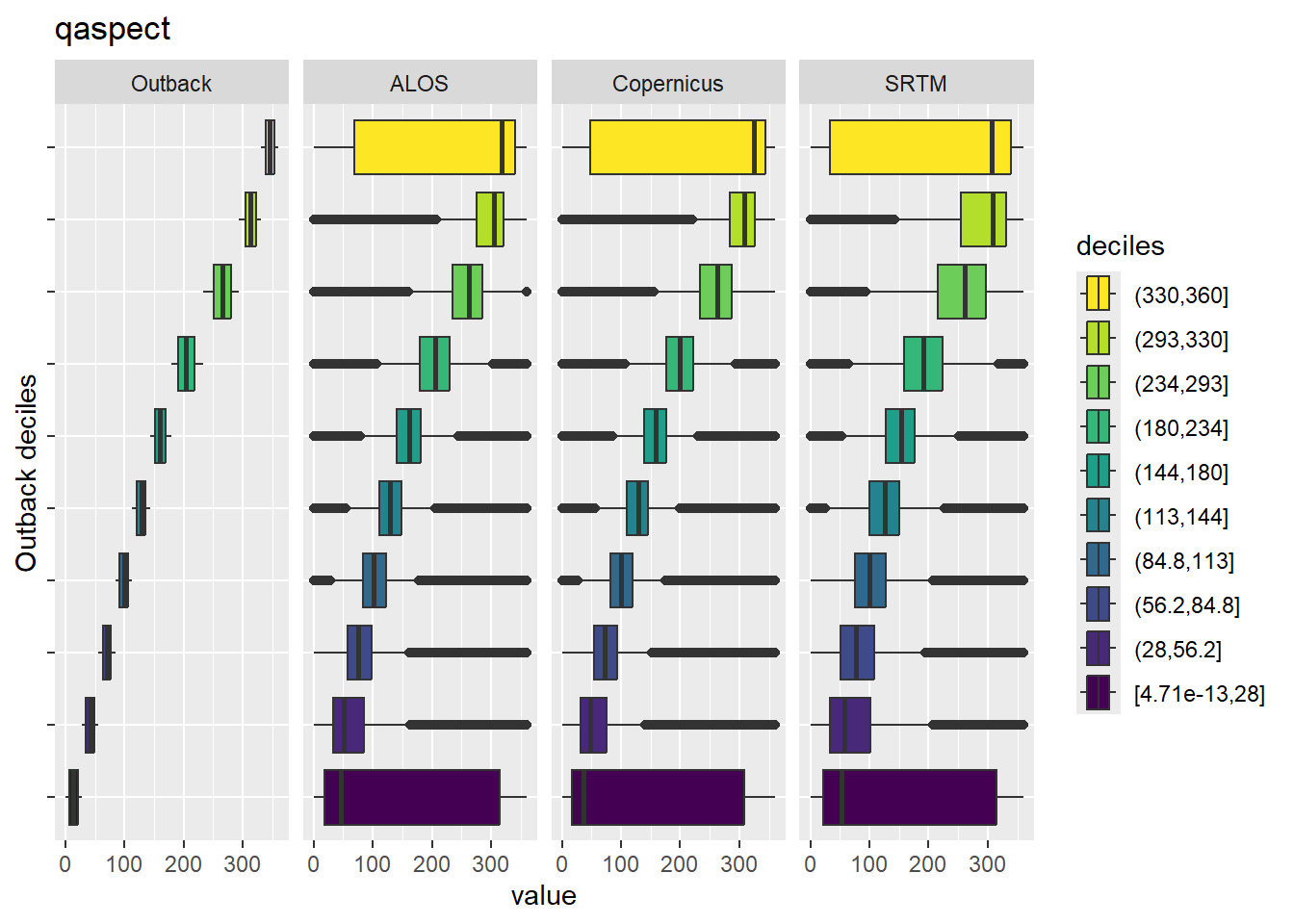
Figure 7.10: Range of values within deciles for each DEM. Deciles are taken from the reference DEM
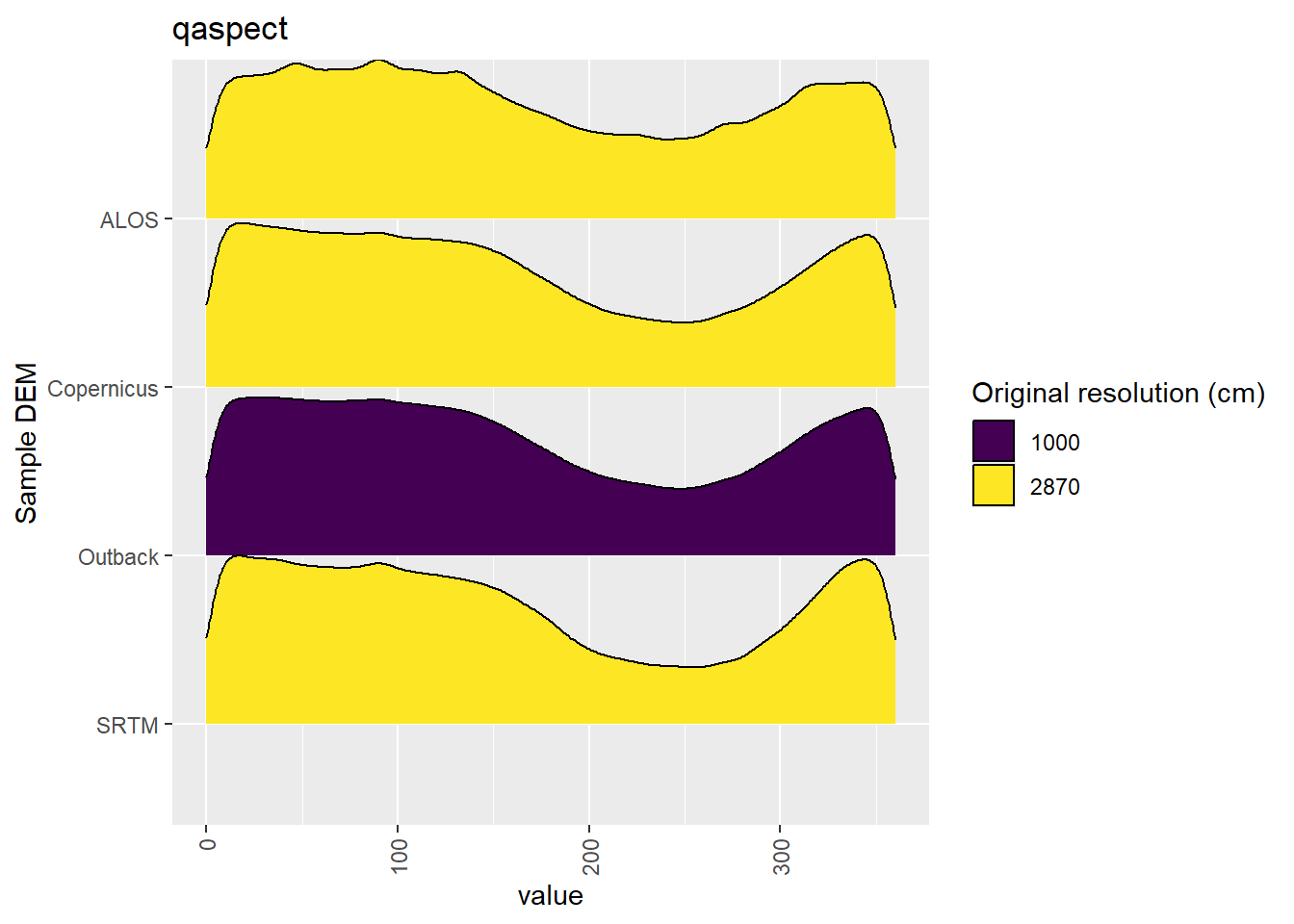
Figure 7.11: Distribution of qaspect values in each DEM: Kanku-Breakaways
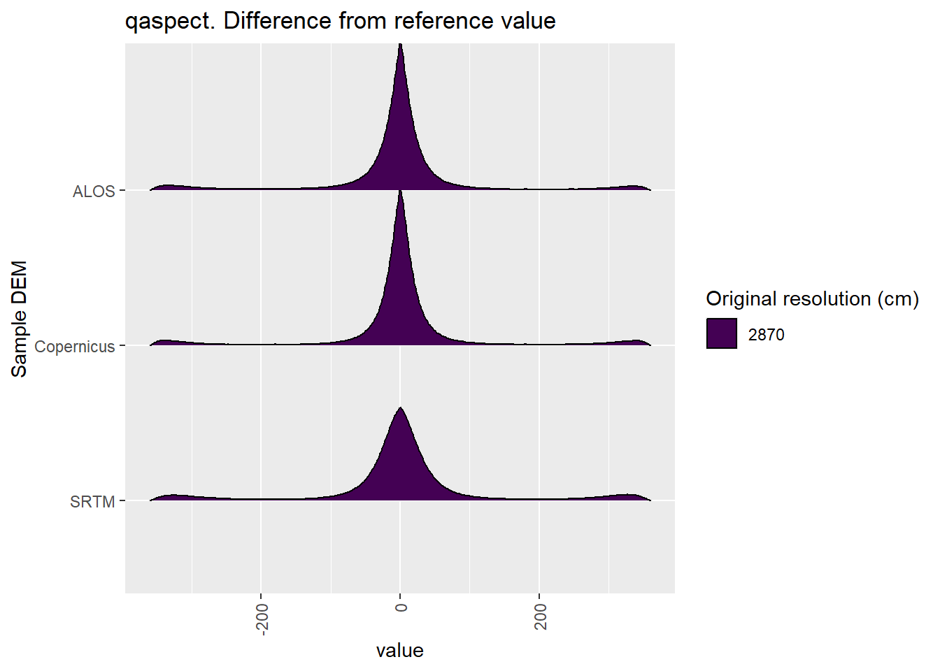
Figure 7.12: Distribution of difference between each DEM and reference for qaspect values: Kanku-Breakaways
7.1.4 qeastness
Figure 7.13 shows rasters for qeastness in the Kanku-Breakaways area.
Table 7.14 shows boxplots for each decile of qeastness, allowing a comparison of values within each DEM across different ranges of qeastness. Deciles are based on the values in the reference DEM: Outback.
Figure 7.15 shows the a distribution of values for each sample DEM and window size.
Figure 7.16 shows the distribution of differences between the reference DEM and the other DEMs.
Figure 7.13: qeastness raster for each DEM
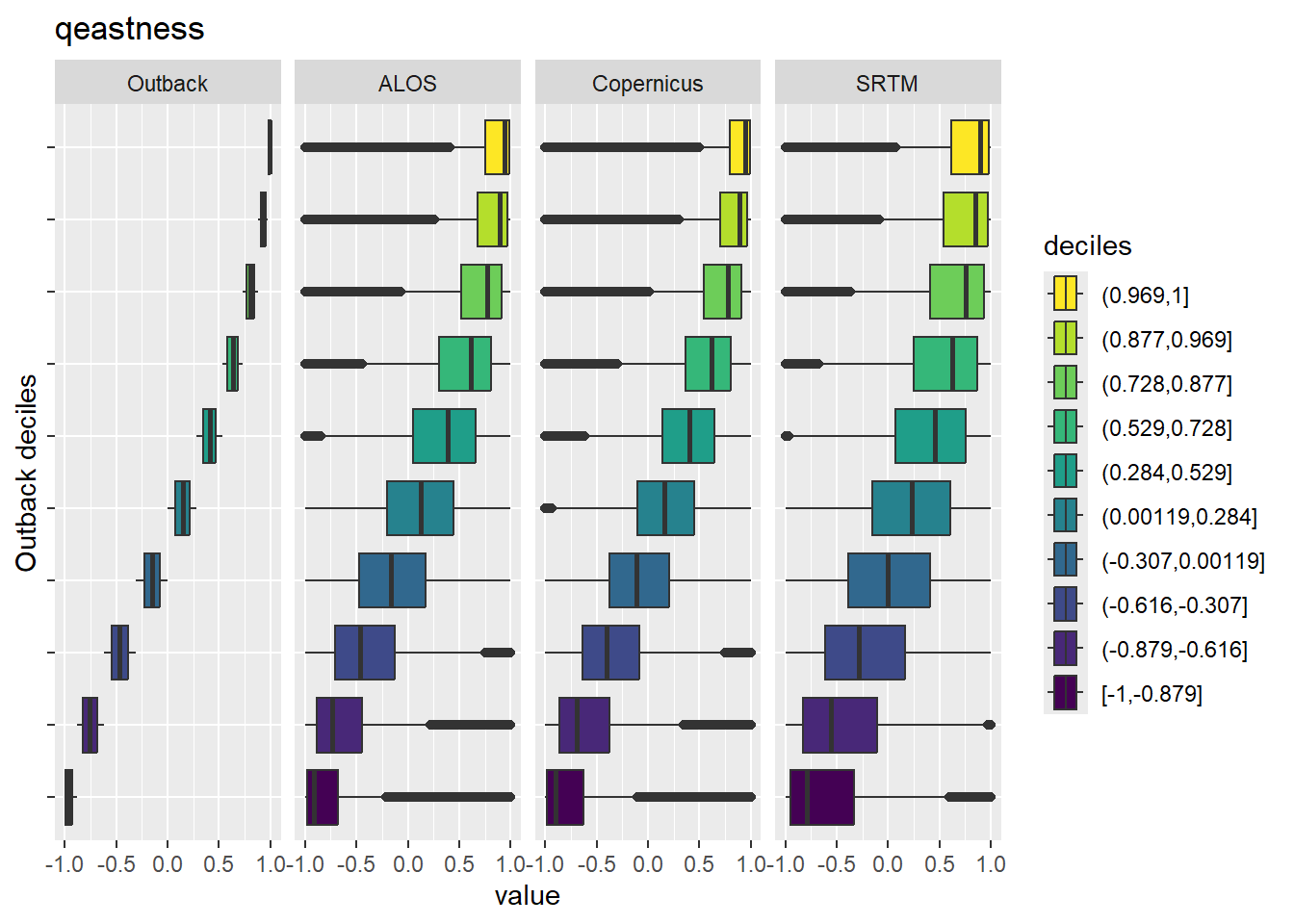
Figure 7.14: Range of values within deciles for each DEM. Deciles are taken from the reference DEM
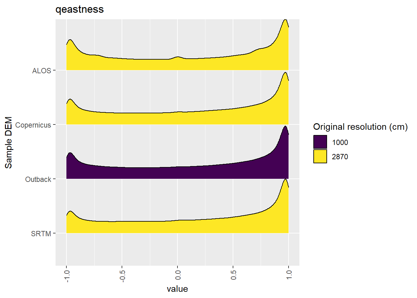
Figure 7.15: Distribution of qeastness values in each DEM: Kanku-Breakaways
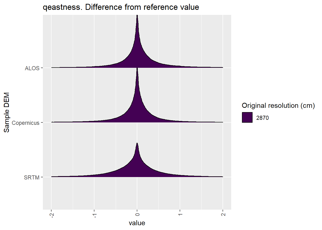
Figure 7.16: Distribution of difference between each DEM and reference for qeastness values: Kanku-Breakaways
7.1.5 qnorthness
Figure 7.17 shows rasters for qnorthness in the Kanku-Breakaways area.
Table 7.18 shows boxplots for each decile of qnorthness, allowing a comparison of values within each DEM across different ranges of qnorthness. Deciles are based on the values in the reference DEM: Outback.
Figure 7.19 shows the a distribution of values for each sample DEM and window size.
Figure 7.20 shows the distribution of differences between the reference DEM and the other DEMs.
Figure 7.17: qnorthness raster for each DEM
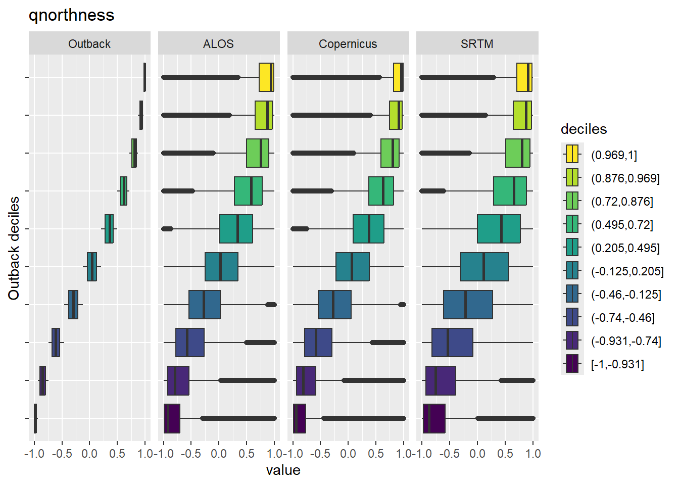
Figure 7.18: Range of values within deciles for each DEM. Deciles are taken from the reference DEM
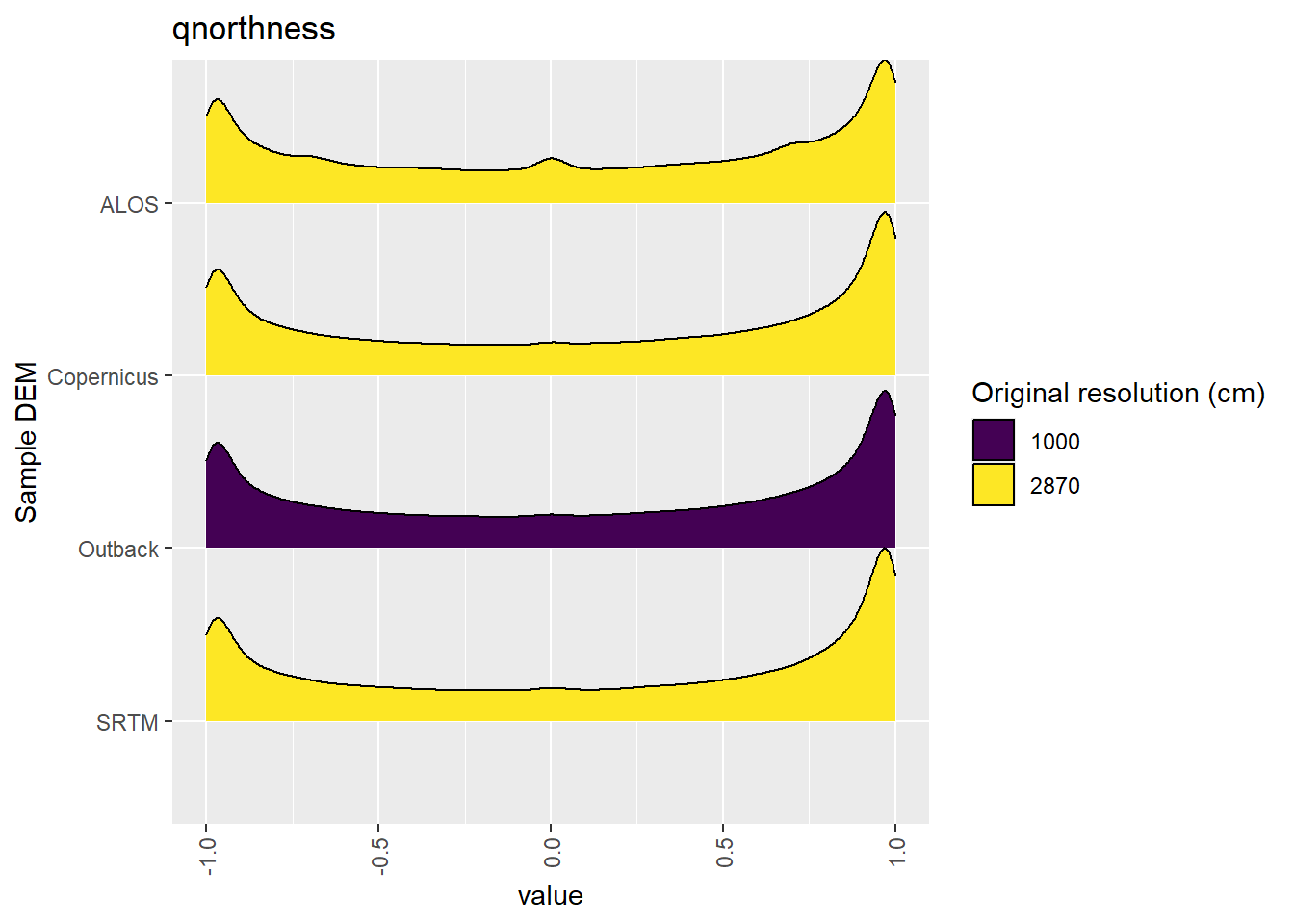
Figure 7.19: Distribution of qnorthness values in each DEM: Kanku-Breakaways
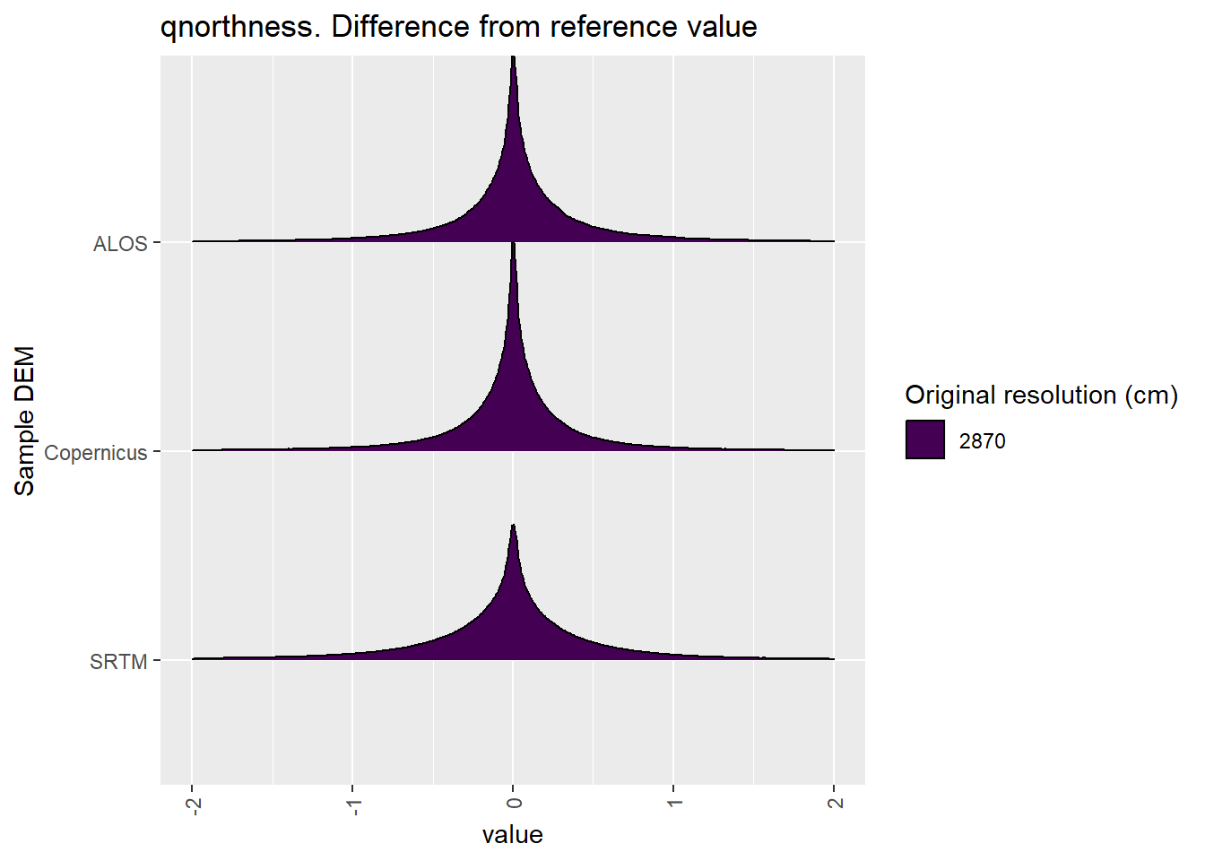
Figure 7.20: Distribution of difference between each DEM and reference for qnorthness values: Kanku-Breakaways
7.1.6 TPI
Figure 7.21 shows rasters for TPI in the Kanku-Breakaways area.
Table 7.22 shows boxplots for each decile of TPI, allowing a comparison of values within each DEM across different ranges of TPI. Deciles are based on the values in the reference DEM: Outback.
Figure 7.23 shows the a distribution of values for each sample DEM and window size.
Figure 7.24 shows the distribution of differences between the reference DEM and the other DEMs.
Figure 7.21: TPI raster for each DEM
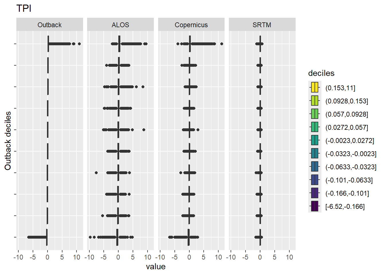
Figure 7.22: Range of values within deciles for each DEM. Deciles are taken from the reference DEM
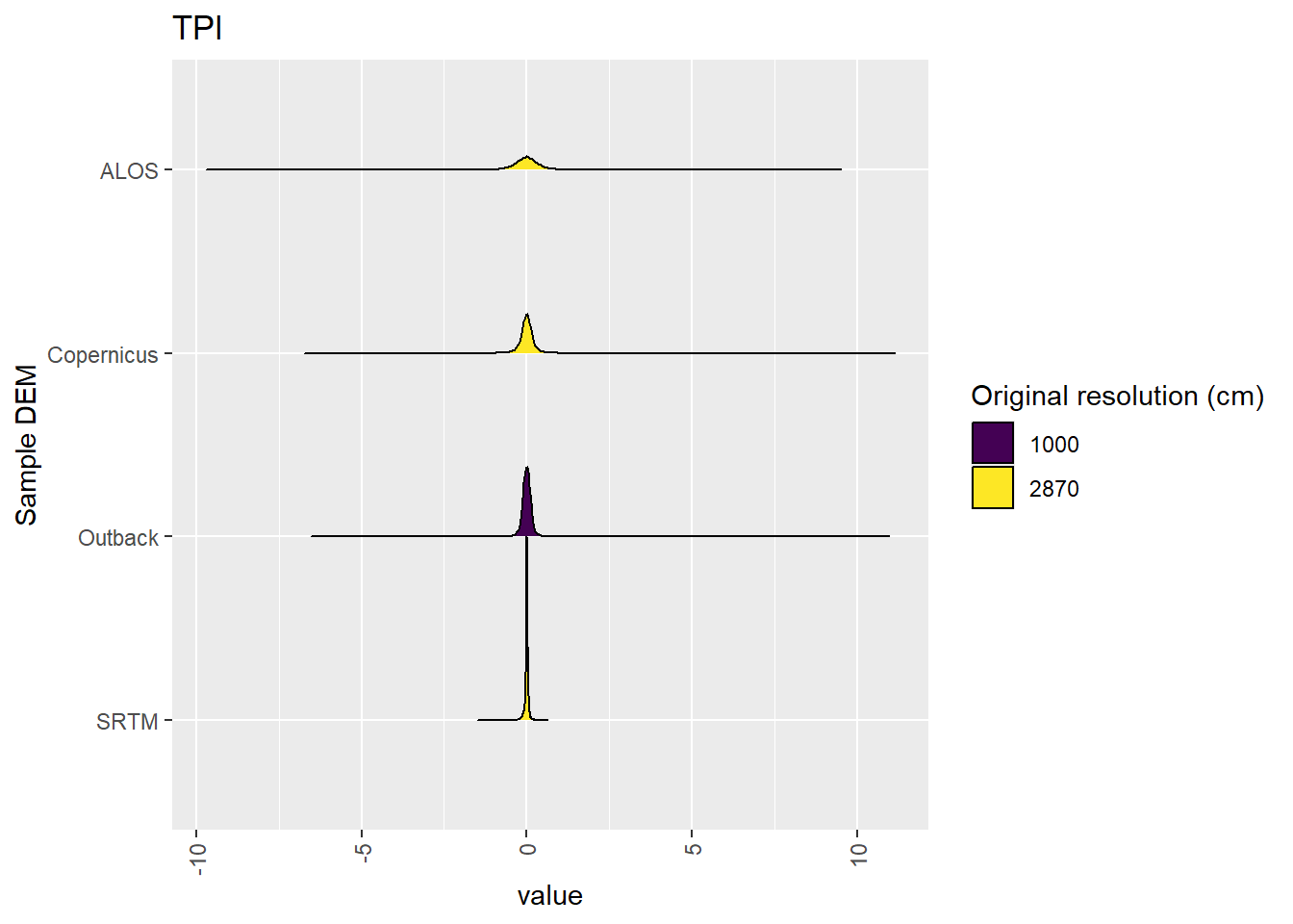
Figure 7.23: Distribution of TPI values in each DEM: Kanku-Breakaways
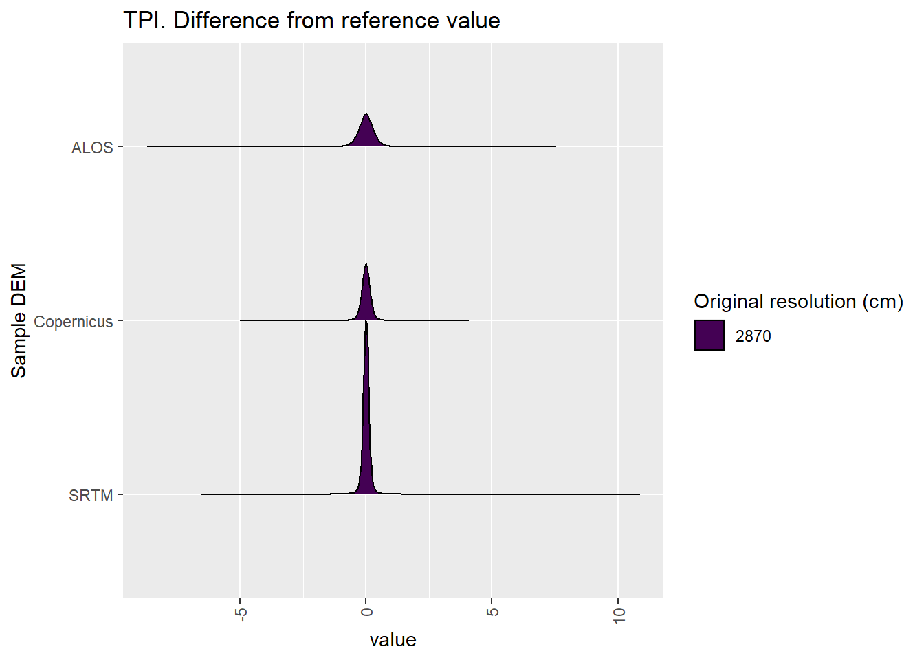
Figure 7.24: Distribution of difference between each DEM and reference for TPI values: Kanku-Breakaways
7.1.7 TRI
Figure 7.25 shows rasters for TRI in the Kanku-Breakaways area.
Table 7.26 shows boxplots for each decile of TRI, allowing a comparison of values within each DEM across different ranges of TRI. Deciles are based on the values in the reference DEM: Outback.
Figure 7.27 shows the a distribution of values for each sample DEM and window size.
Figure 7.28 shows the distribution of differences between the reference DEM and the other DEMs.
Figure 7.25: TRI raster for each DEM
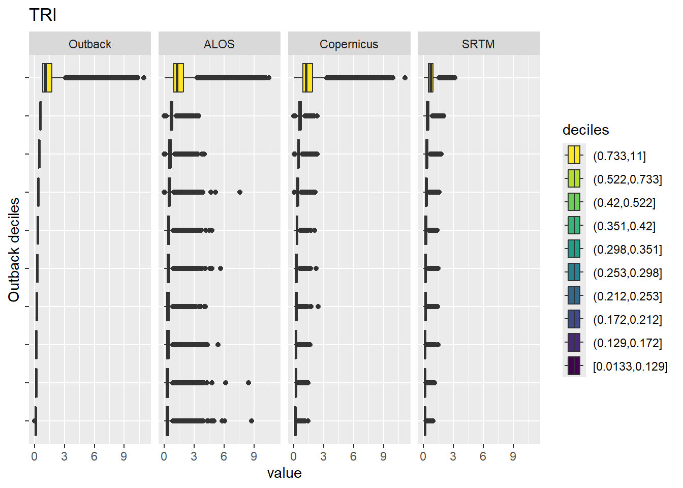
Figure 7.26: Range of values within deciles for each DEM. Deciles are taken from the reference DEM
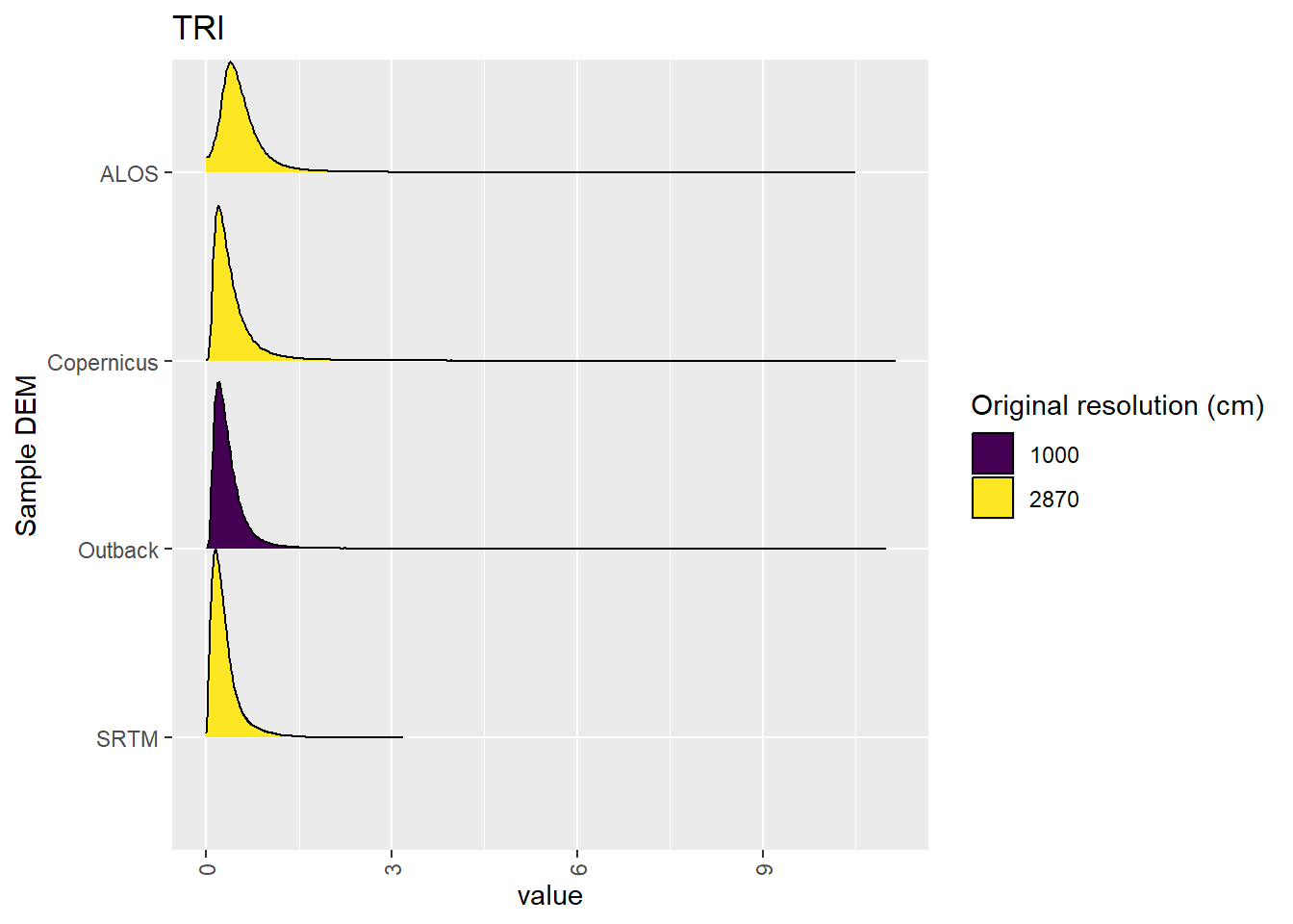
Figure 7.27: Distribution of TRI values in each DEM: Kanku-Breakaways
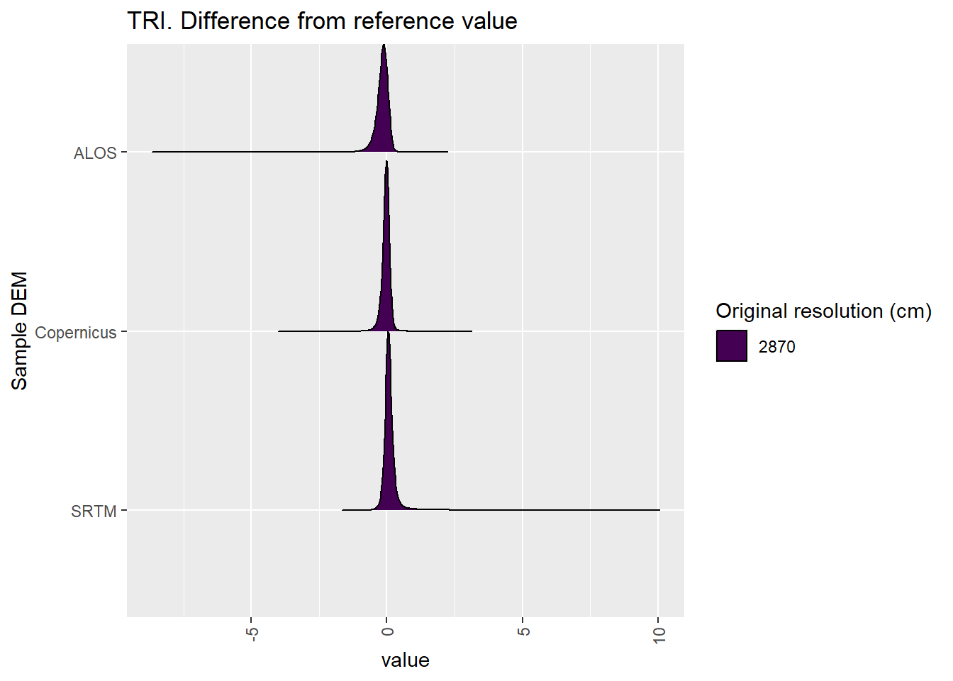
Figure 7.28: Distribution of difference between each DEM and reference for TRI values: Kanku-Breakaways
7.1.8 TRIriley
Figure 7.29 shows rasters for TRIriley in the Kanku-Breakaways area.
Table 7.30 shows boxplots for each decile of TRIriley, allowing a comparison of values within each DEM across different ranges of TRIriley. Deciles are based on the values in the reference DEM: Outback.
Figure 7.31 shows the a distribution of values for each sample DEM and window size.
Figure 7.32 shows the distribution of differences between the reference DEM and the other DEMs.
Figure 7.29: TRIriley raster for each DEM

Figure 7.30: Range of values within deciles for each DEM. Deciles are taken from the reference DEM
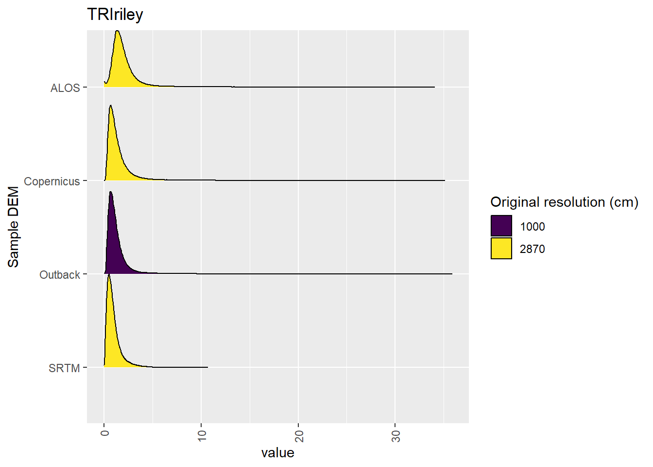
Figure 7.31: Distribution of TRIriley values in each DEM: Kanku-Breakaways
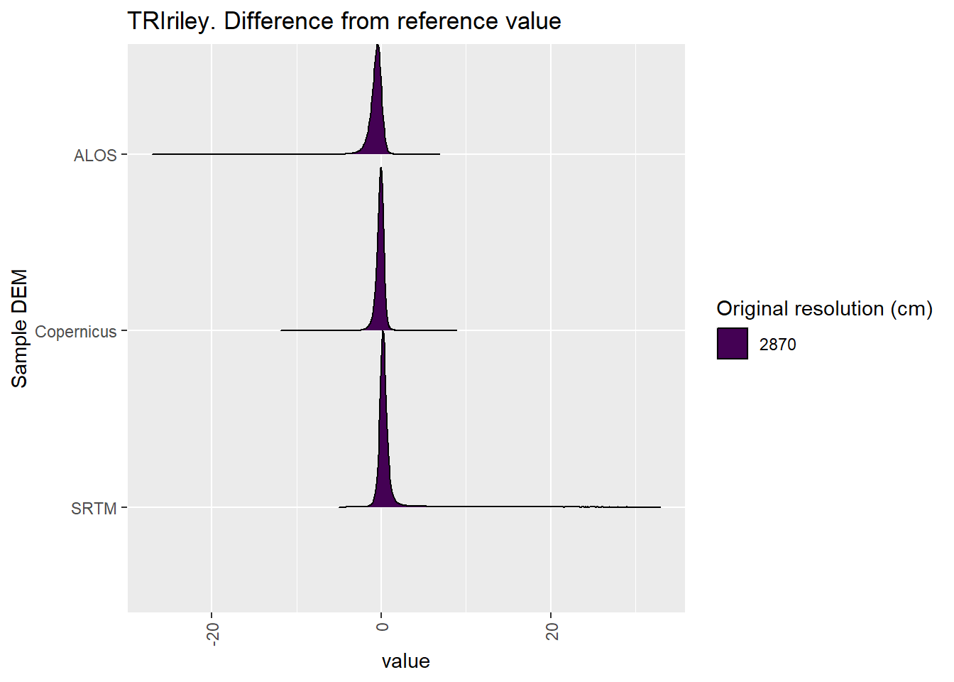
Figure 7.32: Distribution of difference between each DEM and reference for TRIriley values: Kanku-Breakaways
7.1.9 TRIrmsd
Figure 7.33 shows rasters for TRIrmsd in the Kanku-Breakaways area.
Table 7.34 shows boxplots for each decile of TRIrmsd, allowing a comparison of values within each DEM across different ranges of TRIrmsd. Deciles are based on the values in the reference DEM: Outback.
Figure 7.35 shows the a distribution of values for each sample DEM and window size.
Figure 7.36 shows the distribution of differences between the reference DEM and the other DEMs.
Figure 7.33: TRIrmsd raster for each DEM
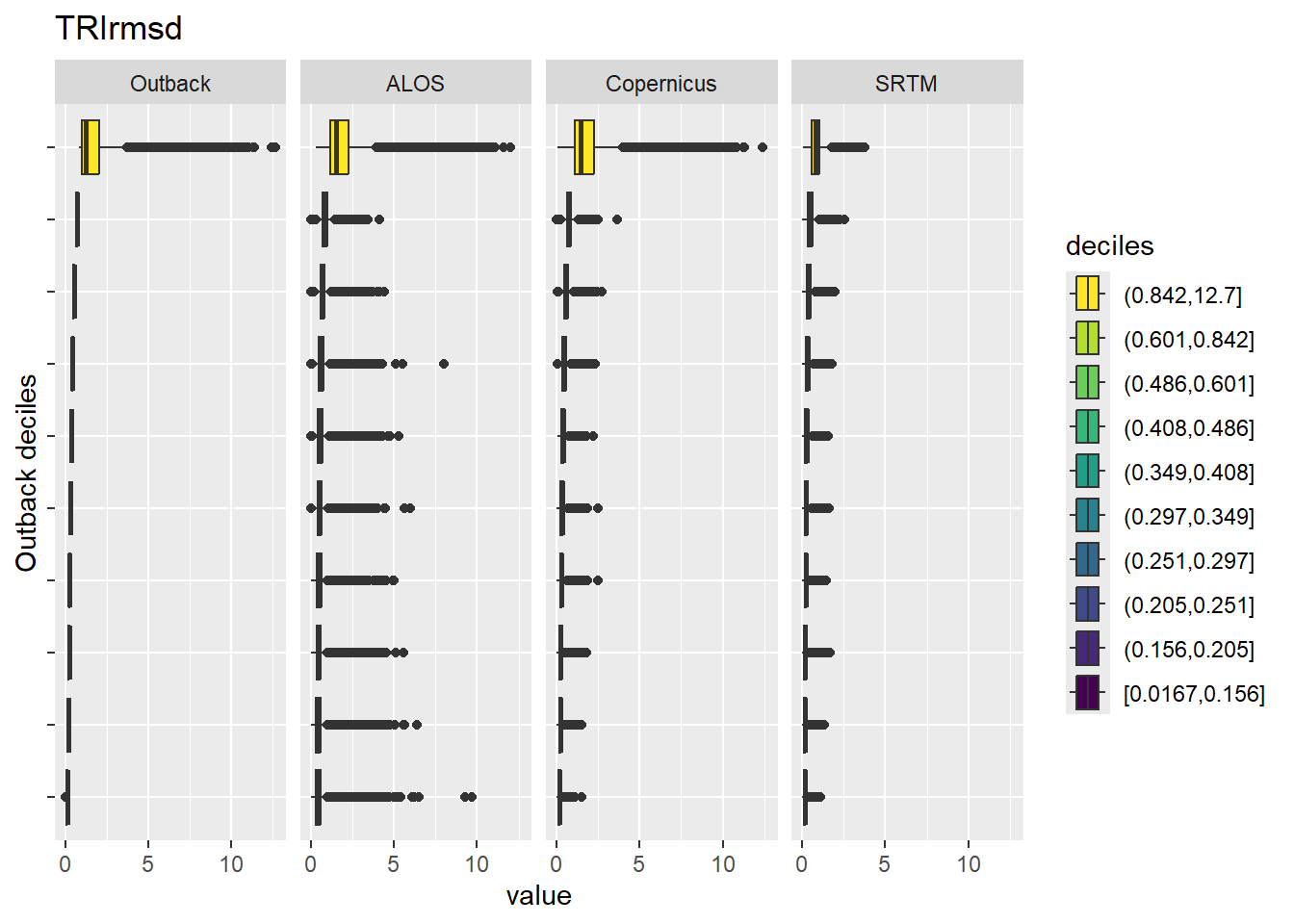
Figure 7.34: Range of values within deciles for each DEM. Deciles are taken from the reference DEM
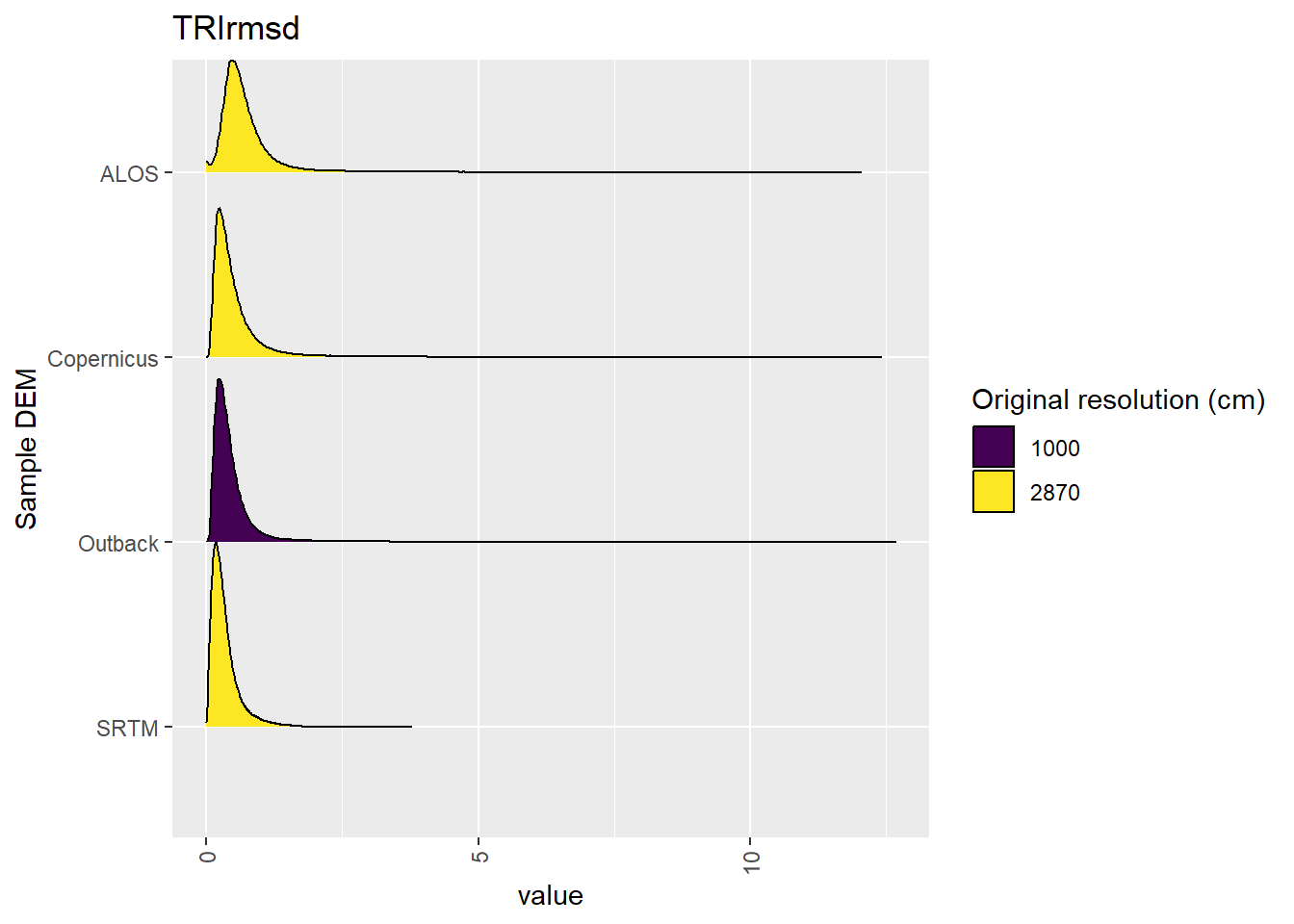
Figure 7.35: Distribution of TRIrmsd values in each DEM: Kanku-Breakaways
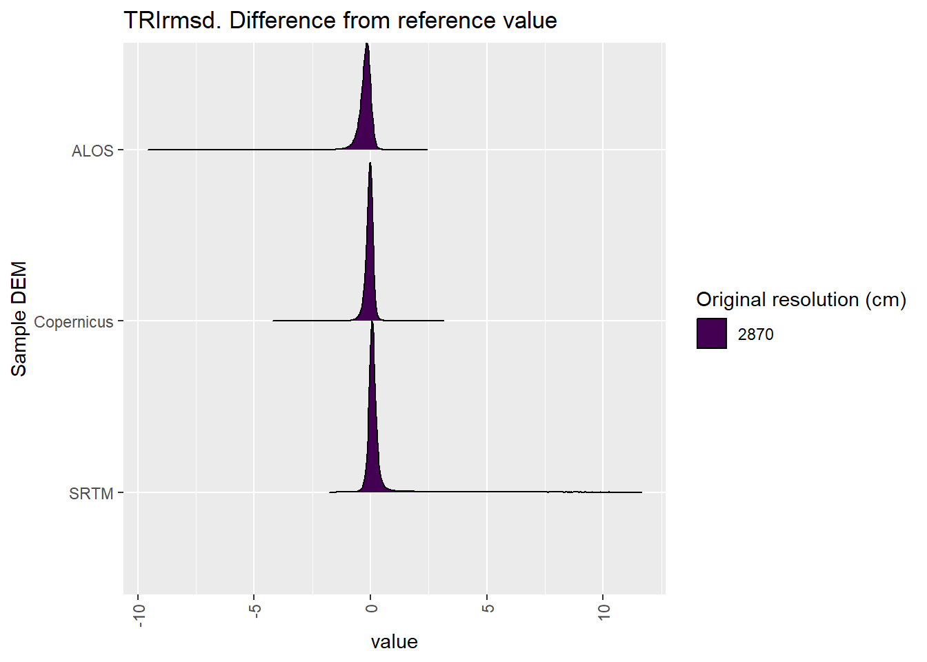
Figure 7.36: Distribution of difference between each DEM and reference for TRIrmsd values: Kanku-Breakaways
7.1.10 roughness
Figure 7.37 shows rasters for roughness in the Kanku-Breakaways area.
Table 7.38 shows boxplots for each decile of roughness, allowing a comparison of values within each DEM across different ranges of roughness. Deciles are based on the values in the reference DEM: Outback.
Figure 7.39 shows the a distribution of values for each sample DEM and window size.
Figure 7.40 shows the distribution of differences between the reference DEM and the other DEMs.
Figure 7.37: roughness raster for each DEM
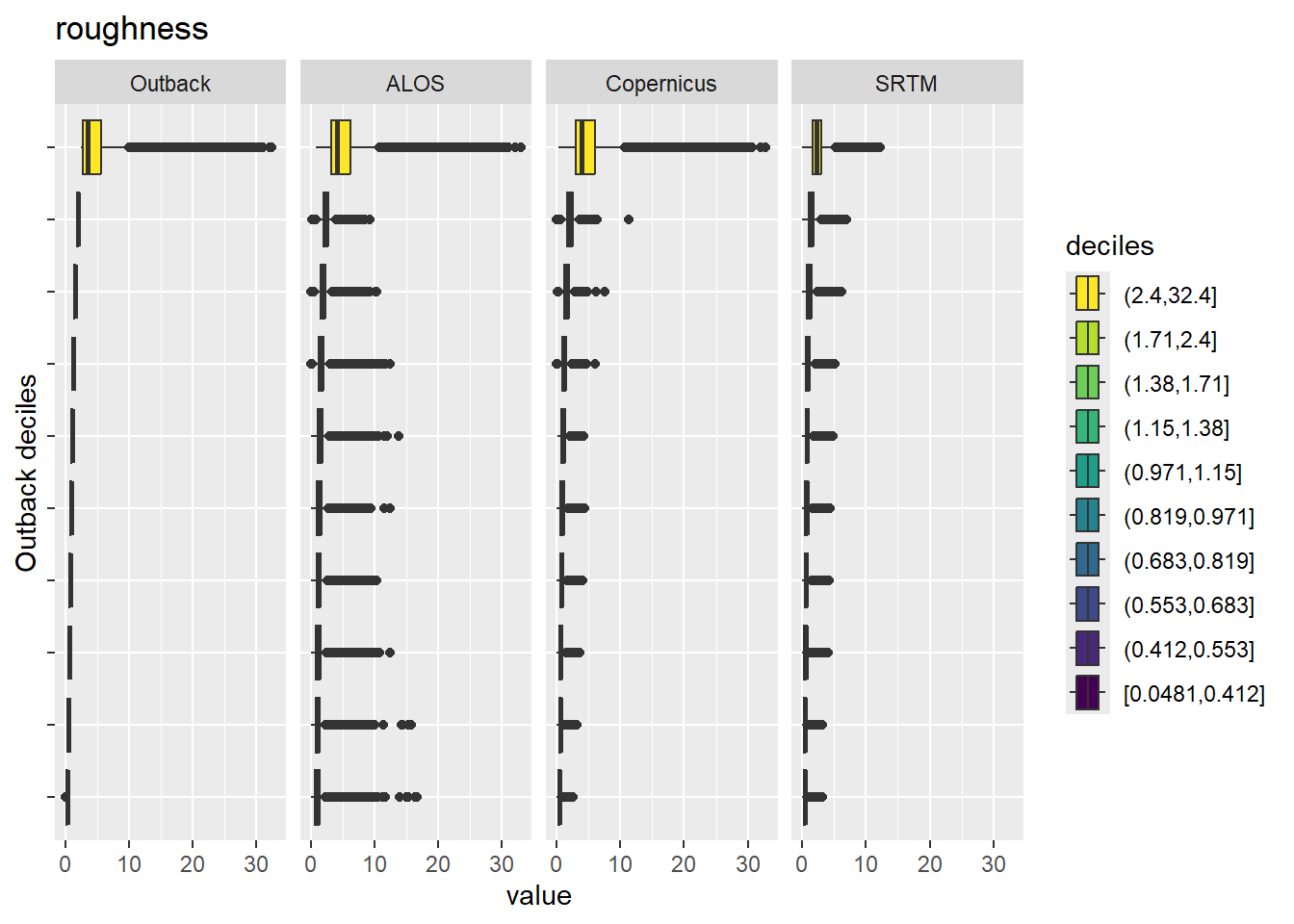
Figure 7.38: Range of values within deciles for each DEM. Deciles are taken from the reference DEM
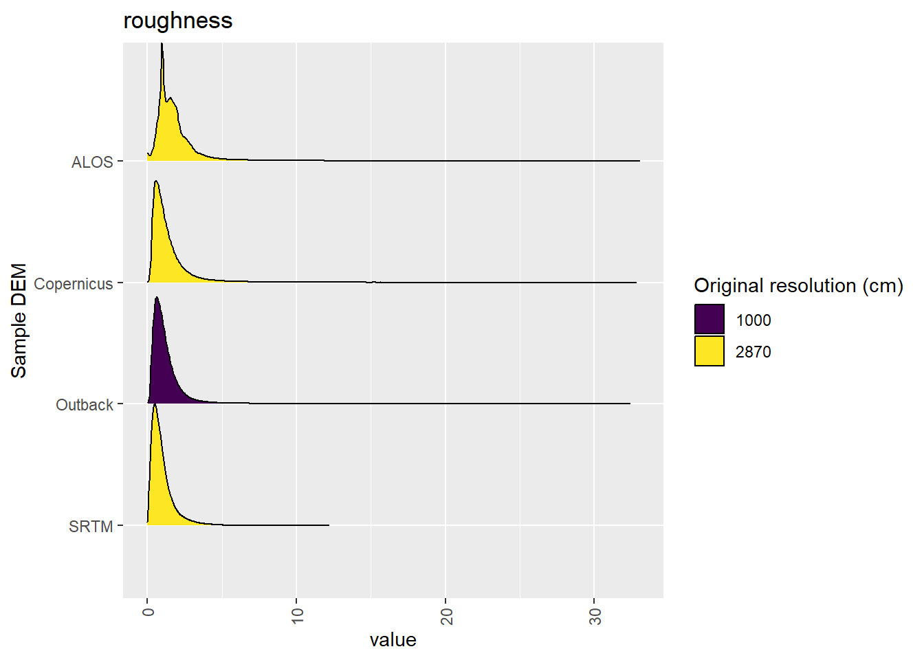
Figure 7.39: Distribution of roughness values in each DEM: Kanku-Breakaways
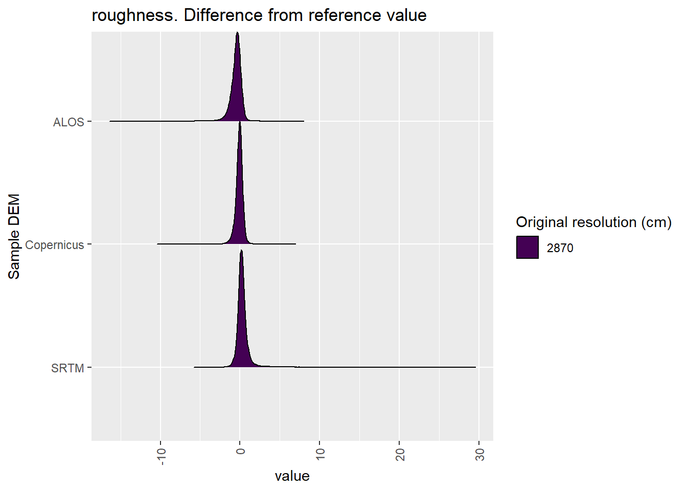
Figure 7.40: Distribution of difference between each DEM and reference for roughness values: Kanku-Breakaways
7.2 Categorical
Table 7.1 shows the proportion of each DEM classifed to each landform element (also see Figure 7.42.
Figure 7.41 shows a landscape classification for each reprojected area.
| landform | Outback | ALOS | Copernicus | SRTM |
|---|---|---|---|---|
| canyon | 0.0065926 | 0.0218612 | 0.009445 | 0.00168 |
| midslope drainage | 0.0081696 | 0.0269690 | 0.017474 | 0.00023 |
| upland drainage | 0.0000020 | 0.0000020 | 0.000011 | |
| u-shaped valley | 0.0288748 | 0.0389482 | 0.024370 | 0.02007 |
| plains | 0.8920463 | 0.8010432 | 0.872433 | 0.96642 |
| open slopes | 0.0151754 | 0.0171155 | 0.016585 | 0.00026 |
| upper slopes | 0.0336745 | 0.0450237 | 0.032529 | 0.01025 |
| local ridges | 0.0000029 | 0.0000049 | 0.000012 | |
| midslopes ridges | 0.0088448 | 0.0273675 | 0.018238 | 0.00016 |
| mountain tops | 0.0066171 | 0.0216649 | 0.008902 | 0.00093 |
Figure 7.41: Categorical representation of Kanku-Breakaways
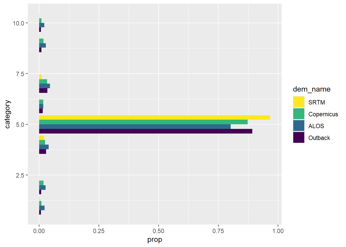
Figure 7.42: Proportion of categorised Kanku-Breakaways area in each of several classification classes