6 Hambidge
6.1 Continuous
6.1.1 elev
Figure 6.1 shows rasters for elev in the Hambidge area.
Table 6.2 shows boxplots for each decile of elev, allowing a comparison of values within each DEM across different ranges of elev. Deciles are based on the values in the reference DEM: Ag.
Figure 6.3 shows the a distribution of values for each sample DEM and window size.
Figure 6.4 shows the distribution of differences between the reference DEM and the other DEMs.
Figure 6.1: elev raster for each DEM
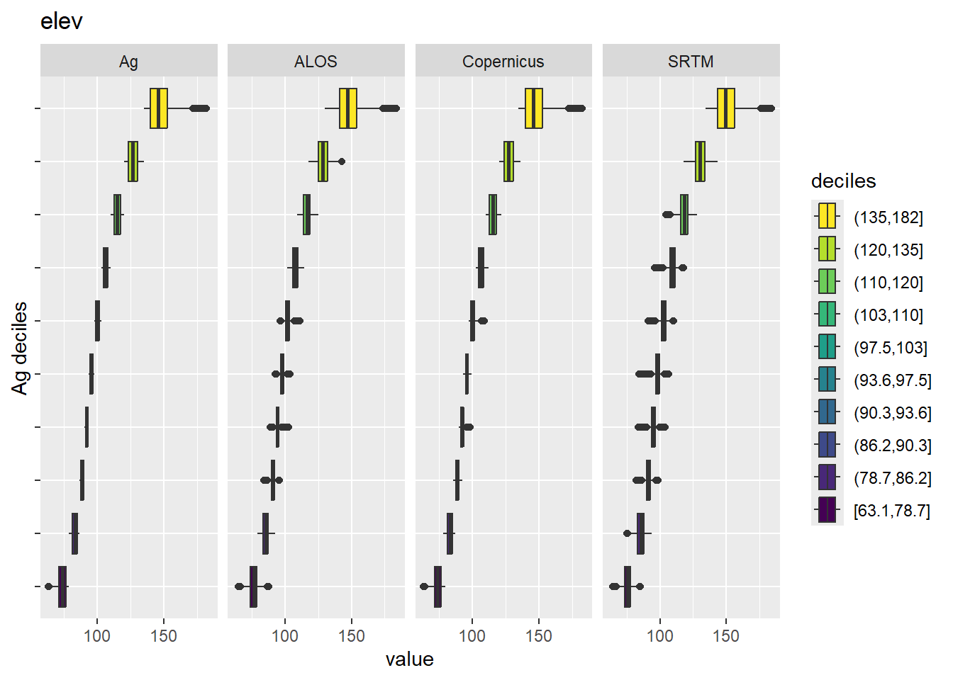
Figure 6.2: Range of values within deciles for each DEM. Deciles are taken from the reference DEM
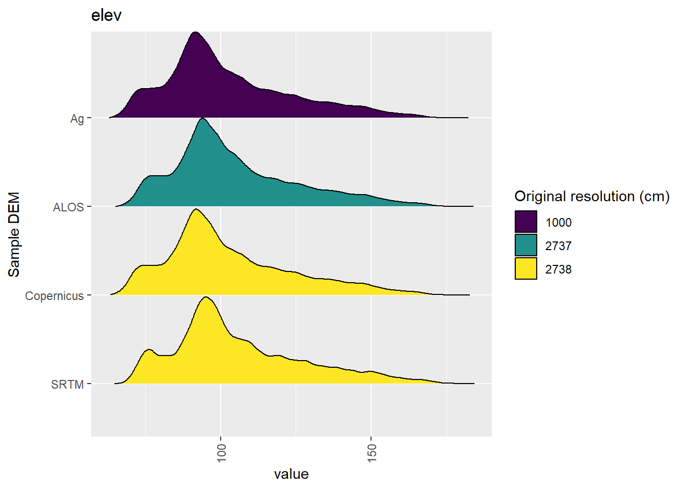
Figure 6.3: Distribution of elev values in each DEM: Hambidge
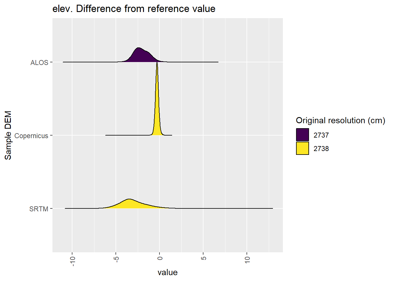
Figure 6.4: Distribution of difference between each DEM and reference for elev values: Hambidge
6.1.2 qslope
Figure 6.5 shows rasters for qslope in the Hambidge area.
Table 6.6 shows boxplots for each decile of qslope, allowing a comparison of values within each DEM across different ranges of qslope. Deciles are based on the values in the reference DEM: Ag.
Figure 6.7 shows the a distribution of values for each sample DEM and window size.
Figure 6.8 shows the distribution of differences between the reference DEM and the other DEMs.
Figure 6.5: qslope raster for each DEM
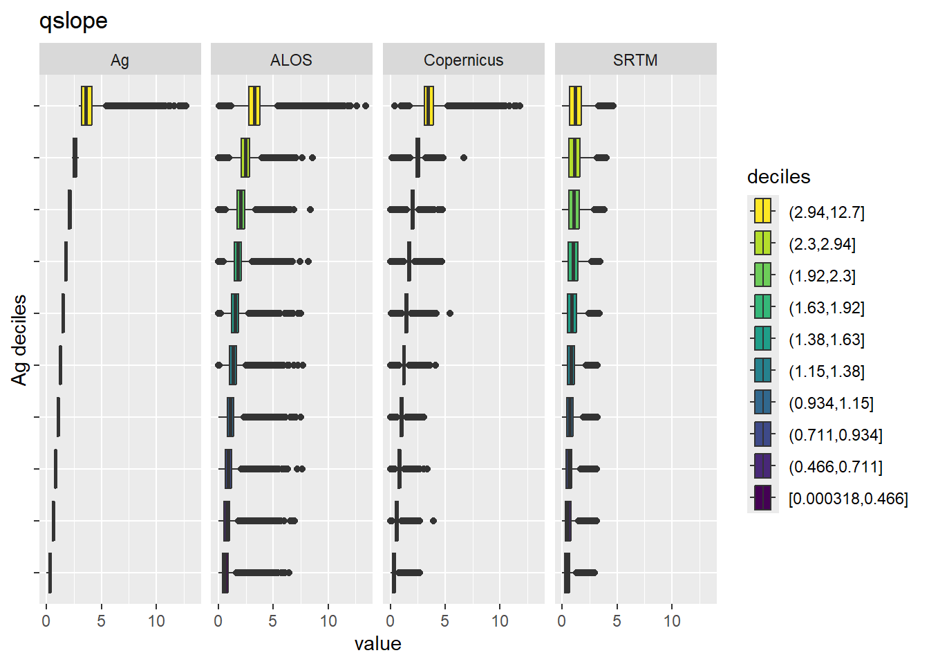
Figure 6.6: Range of values within deciles for each DEM. Deciles are taken from the reference DEM
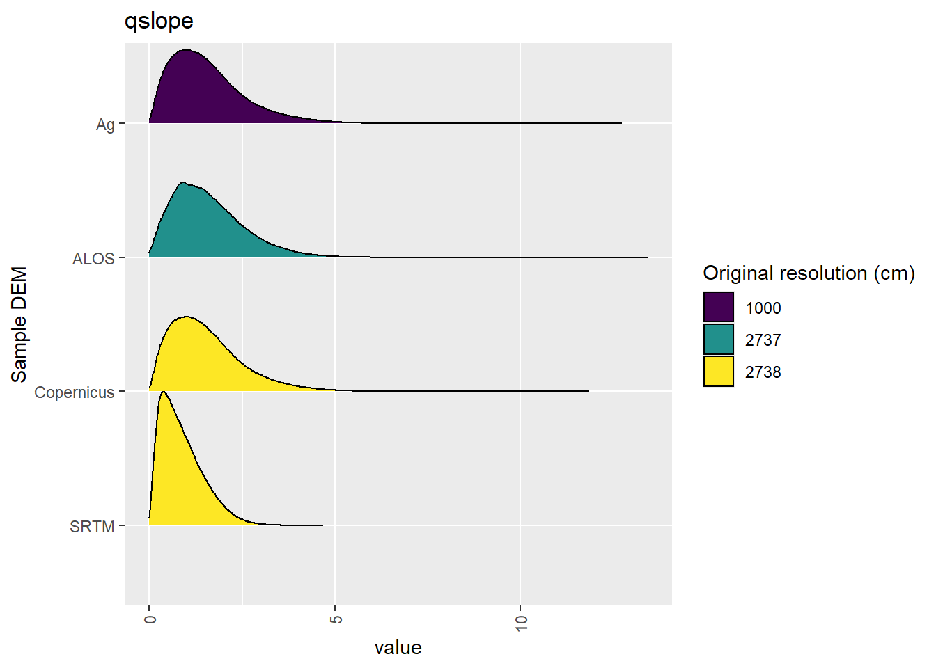
Figure 6.7: Distribution of qslope values in each DEM: Hambidge
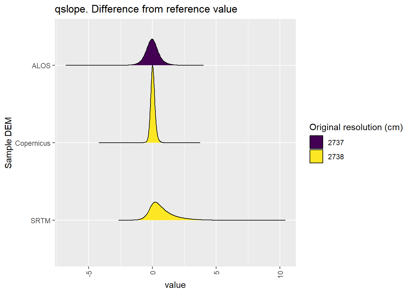
Figure 6.8: Distribution of difference between each DEM and reference for qslope values: Hambidge
6.1.3 qaspect
Figure 6.9 shows rasters for qaspect in the Hambidge area.
Table 6.10 shows boxplots for each decile of qaspect, allowing a comparison of values within each DEM across different ranges of qaspect. Deciles are based on the values in the reference DEM: Ag.
Figure 6.11 shows the a distribution of values for each sample DEM and window size.
Figure 6.12 shows the distribution of differences between the reference DEM and the other DEMs.
Figure 6.9: qaspect raster for each DEM
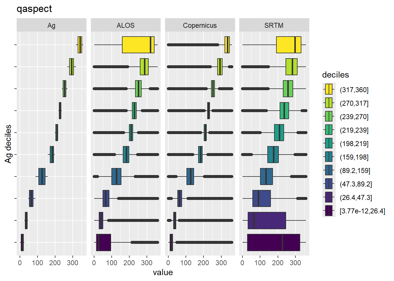
Figure 6.10: Range of values within deciles for each DEM. Deciles are taken from the reference DEM
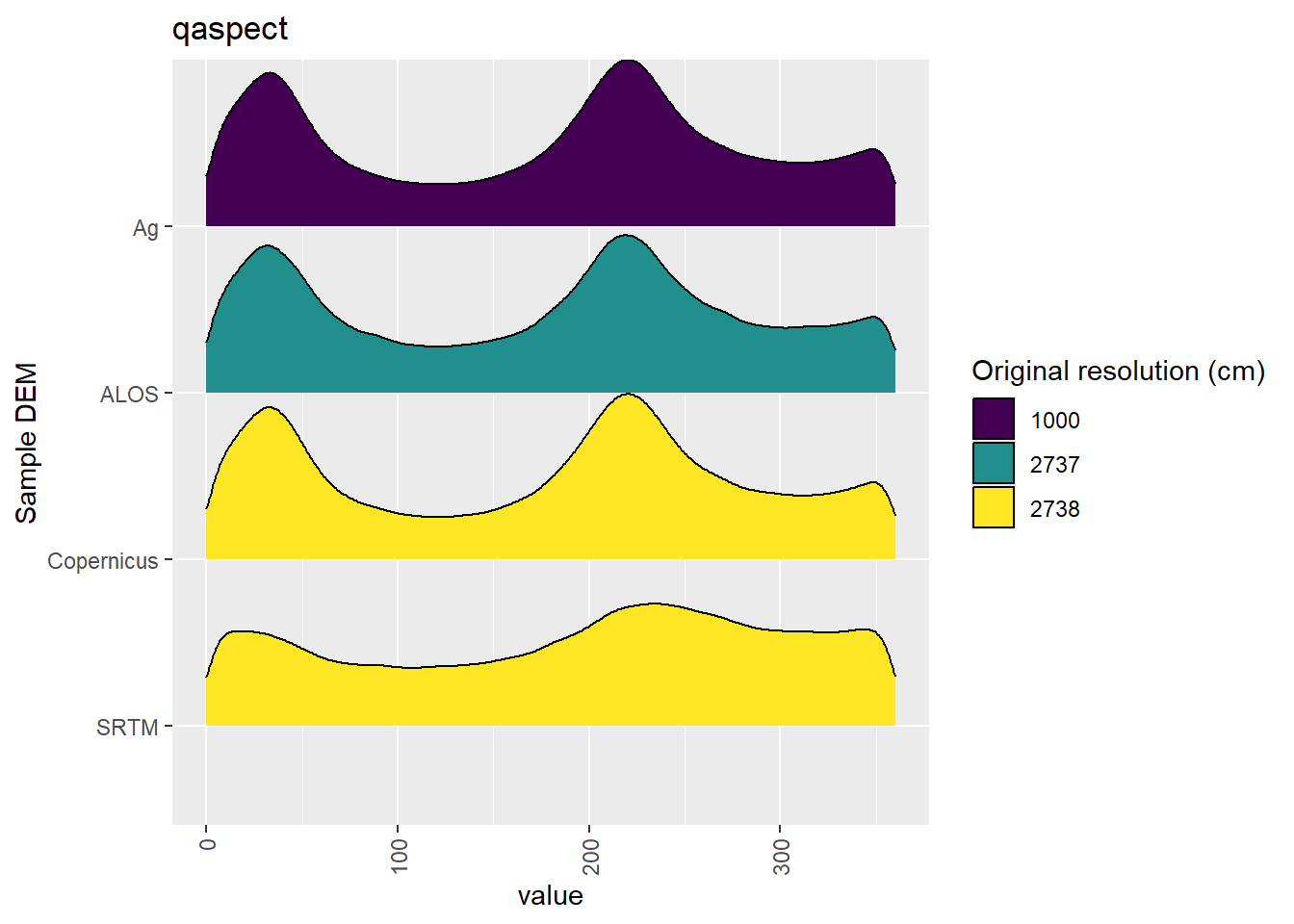
Figure 6.11: Distribution of qaspect values in each DEM: Hambidge
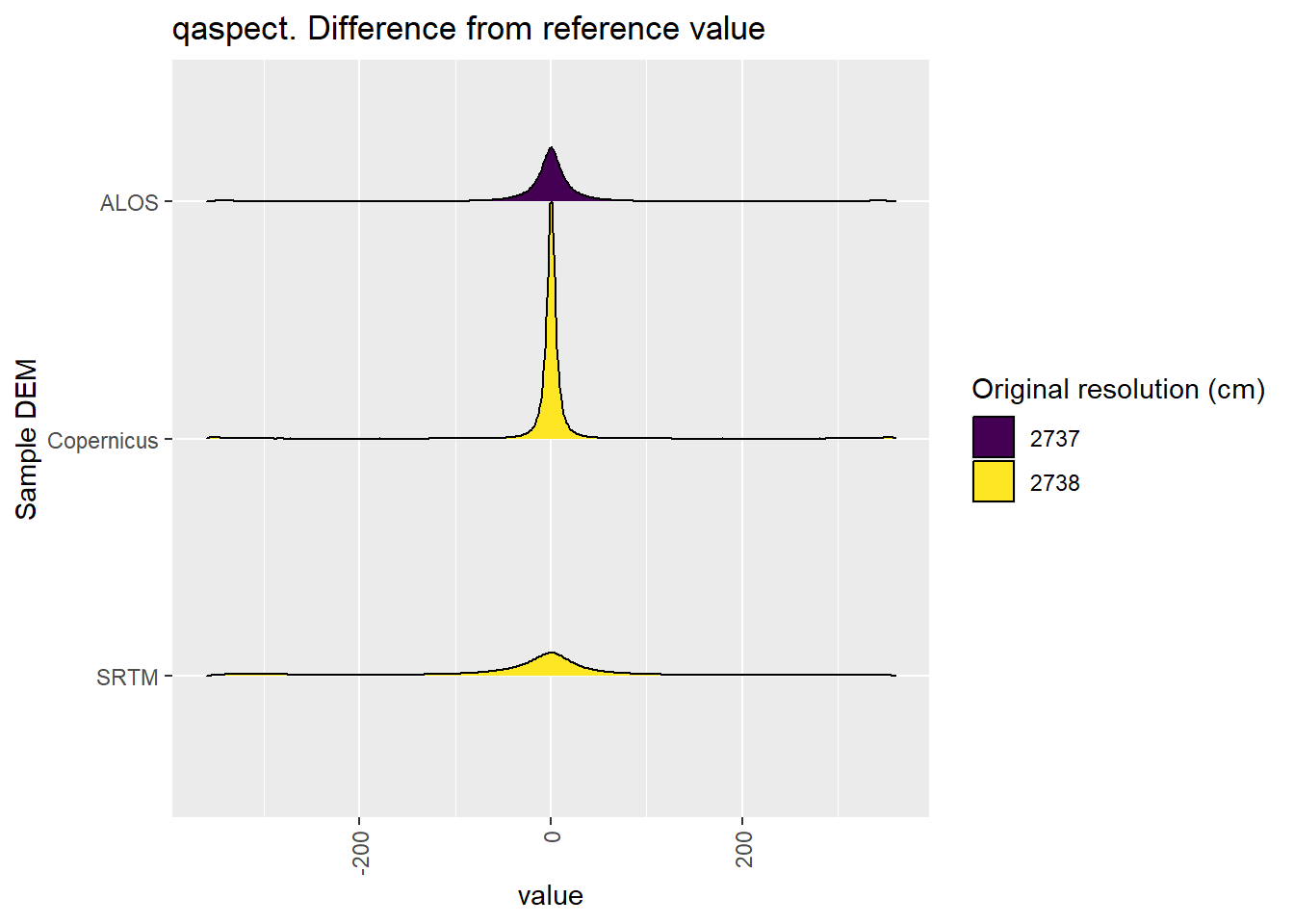
Figure 6.12: Distribution of difference between each DEM and reference for qaspect values: Hambidge
6.1.4 qeastness
Figure 6.13 shows rasters for qeastness in the Hambidge area.
Table 6.14 shows boxplots for each decile of qeastness, allowing a comparison of values within each DEM across different ranges of qeastness. Deciles are based on the values in the reference DEM: Ag.
Figure 6.15 shows the a distribution of values for each sample DEM and window size.
Figure 6.16 shows the distribution of differences between the reference DEM and the other DEMs.
Figure 6.13: qeastness raster for each DEM
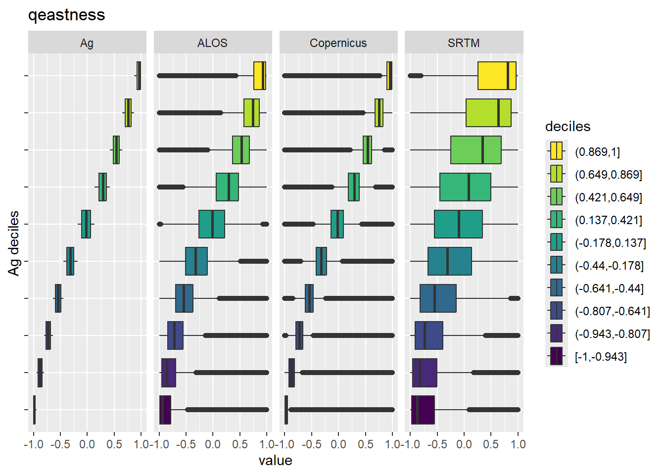
Figure 6.14: Range of values within deciles for each DEM. Deciles are taken from the reference DEM
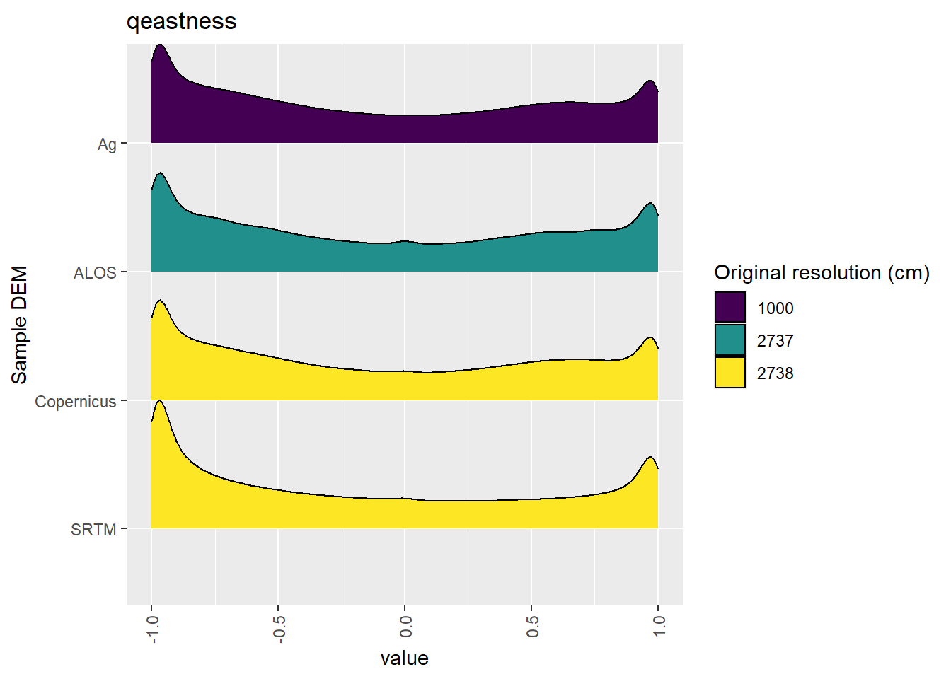
Figure 6.15: Distribution of qeastness values in each DEM: Hambidge
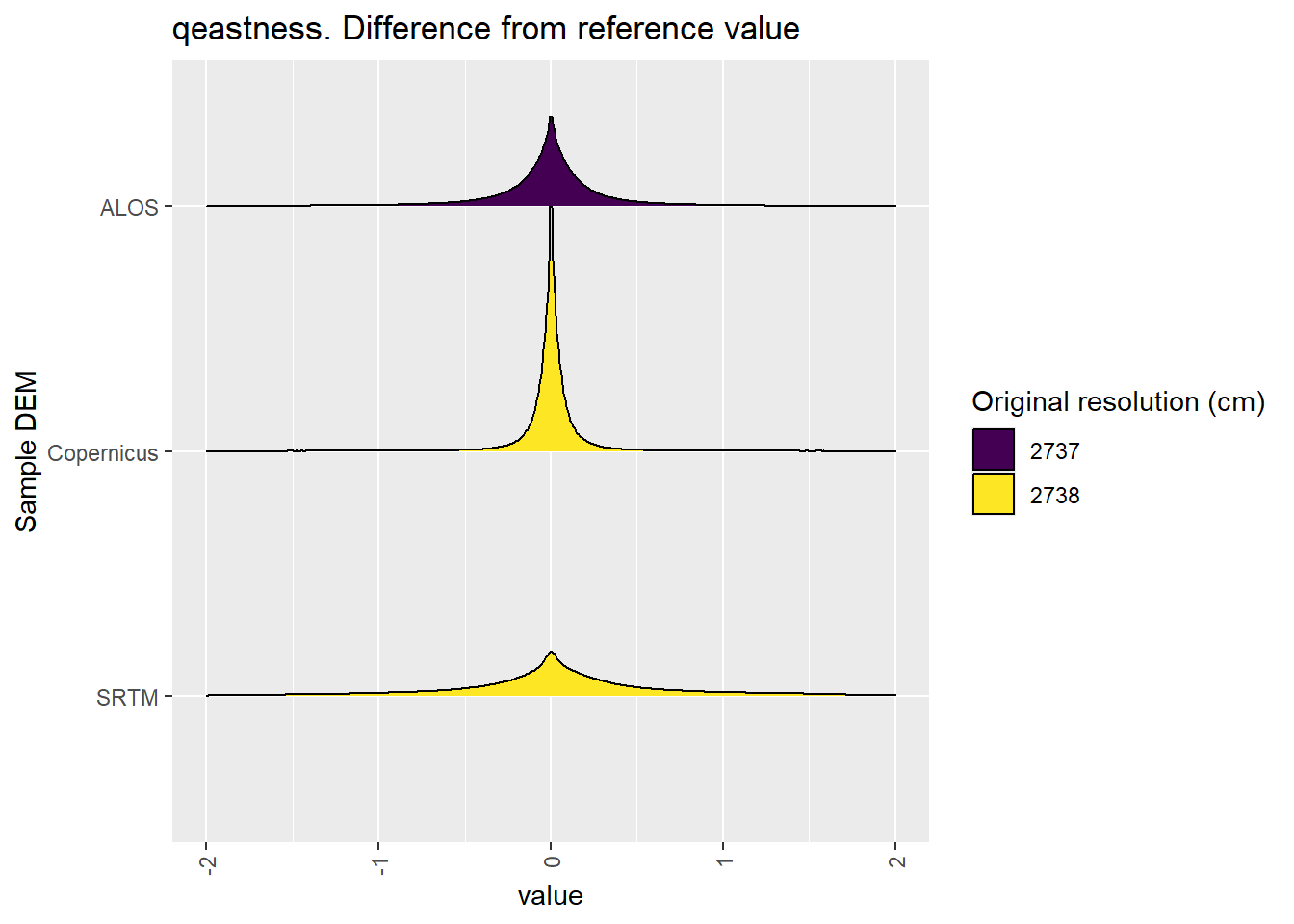
Figure 6.16: Distribution of difference between each DEM and reference for qeastness values: Hambidge
6.1.5 qnorthness
Figure 6.17 shows rasters for qnorthness in the Hambidge area.
Table 6.18 shows boxplots for each decile of qnorthness, allowing a comparison of values within each DEM across different ranges of qnorthness. Deciles are based on the values in the reference DEM: Ag.
Figure 6.19 shows the a distribution of values for each sample DEM and window size.
Figure 6.20 shows the distribution of differences between the reference DEM and the other DEMs.
Figure 6.17: qnorthness raster for each DEM
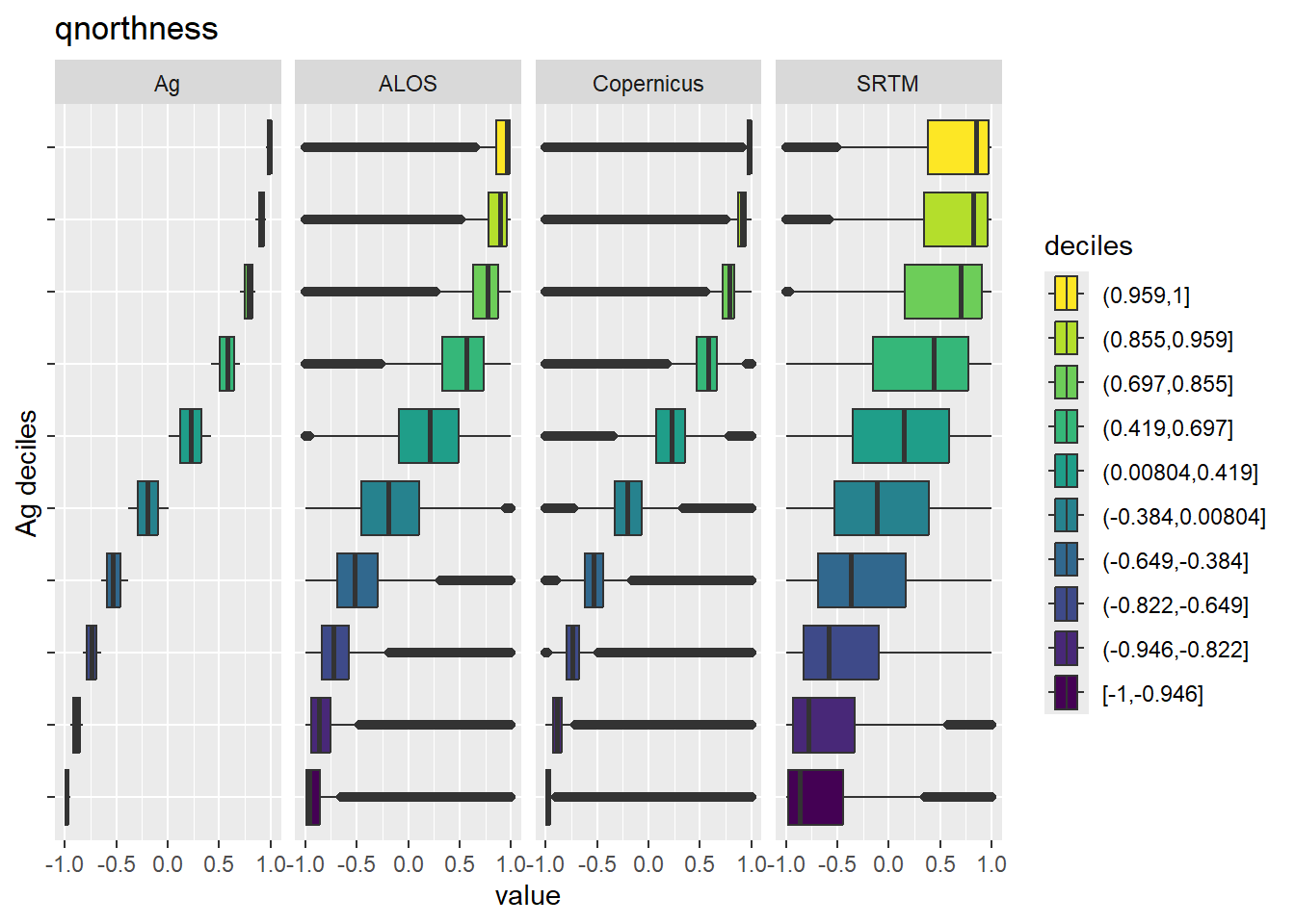
Figure 6.18: Range of values within deciles for each DEM. Deciles are taken from the reference DEM
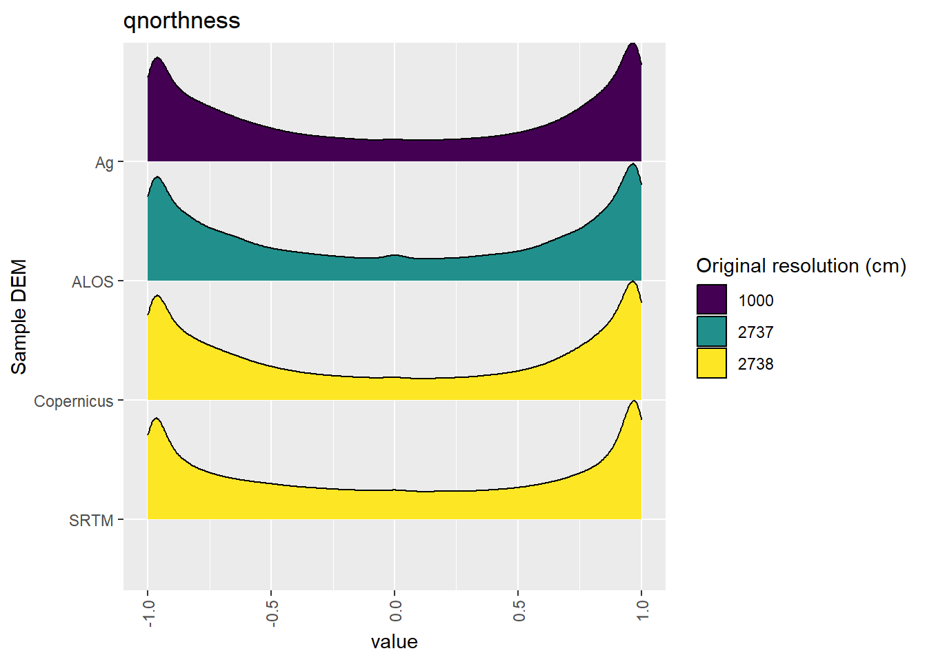
Figure 6.19: Distribution of qnorthness values in each DEM: Hambidge
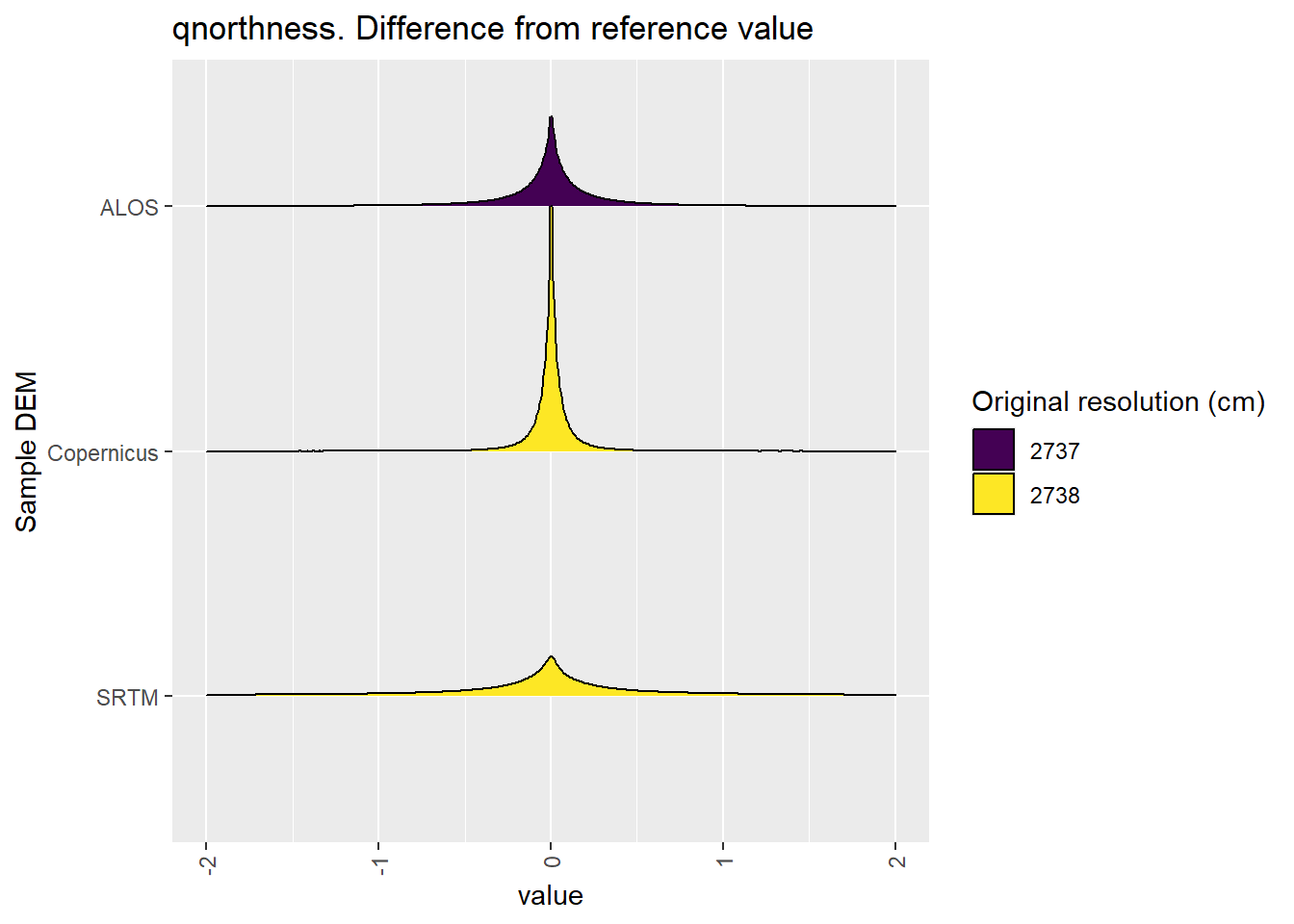
Figure 6.20: Distribution of difference between each DEM and reference for qnorthness values: Hambidge
6.1.6 TPI
Figure 6.21 shows rasters for TPI in the Hambidge area.
Table 6.22 shows boxplots for each decile of TPI, allowing a comparison of values within each DEM across different ranges of TPI. Deciles are based on the values in the reference DEM: Ag.
Figure 6.23 shows the a distribution of values for each sample DEM and window size.
Figure 6.24 shows the distribution of differences between the reference DEM and the other DEMs.
Figure 6.21: TPI raster for each DEM
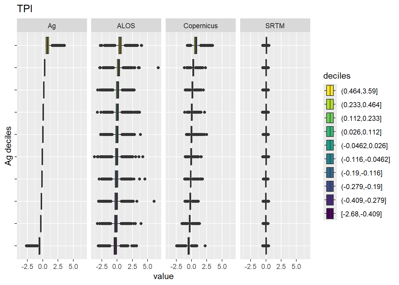
Figure 6.22: Range of values within deciles for each DEM. Deciles are taken from the reference DEM
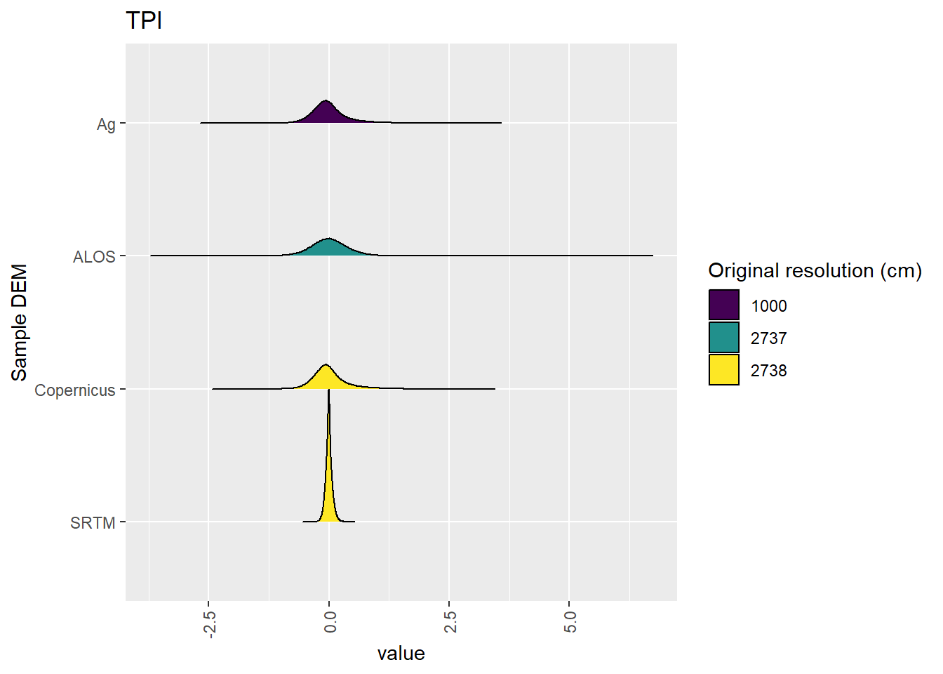
Figure 6.23: Distribution of TPI values in each DEM: Hambidge
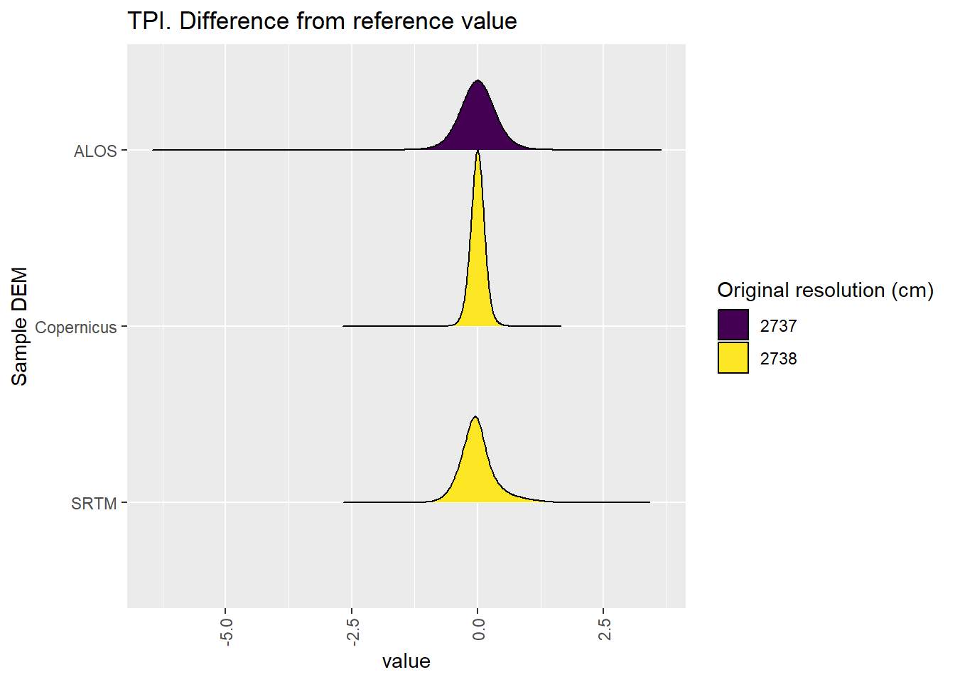
Figure 6.24: Distribution of difference between each DEM and reference for TPI values: Hambidge
6.1.7 TRI
Figure 6.25 shows rasters for TRI in the Hambidge area.
Table 6.26 shows boxplots for each decile of TRI, allowing a comparison of values within each DEM across different ranges of TRI. Deciles are based on the values in the reference DEM: Ag.
Figure 6.27 shows the a distribution of values for each sample DEM and window size.
Figure 6.28 shows the distribution of differences between the reference DEM and the other DEMs.
Figure 6.25: TRI raster for each DEM
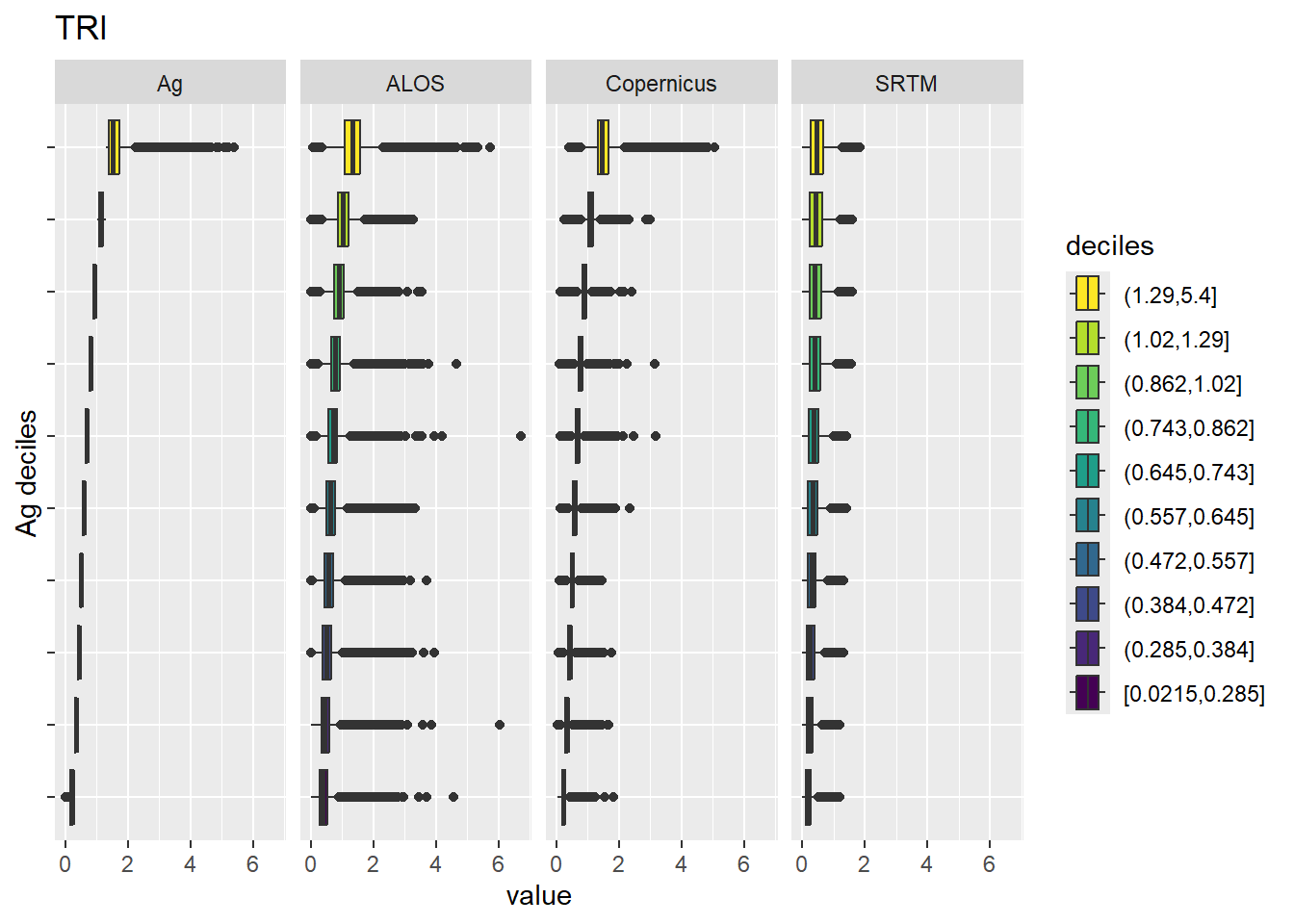
Figure 6.26: Range of values within deciles for each DEM. Deciles are taken from the reference DEM
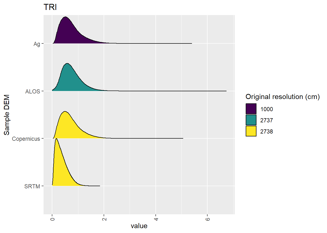
Figure 6.27: Distribution of TRI values in each DEM: Hambidge
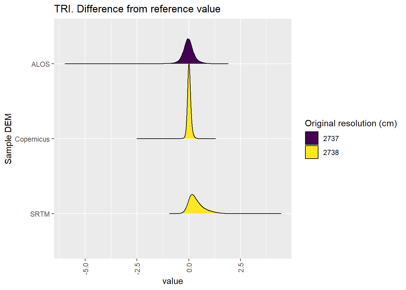
Figure 6.28: Distribution of difference between each DEM and reference for TRI values: Hambidge
6.1.8 TRIriley
Figure 6.29 shows rasters for TRIriley in the Hambidge area.
Table 6.30 shows boxplots for each decile of TRIriley, allowing a comparison of values within each DEM across different ranges of TRIriley. Deciles are based on the values in the reference DEM: Ag.
Figure 6.31 shows the a distribution of values for each sample DEM and window size.
Figure 6.32 shows the distribution of differences between the reference DEM and the other DEMs.
Figure 6.29: TRIriley raster for each DEM
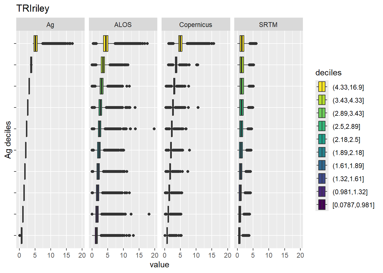
Figure 6.30: Range of values within deciles for each DEM. Deciles are taken from the reference DEM
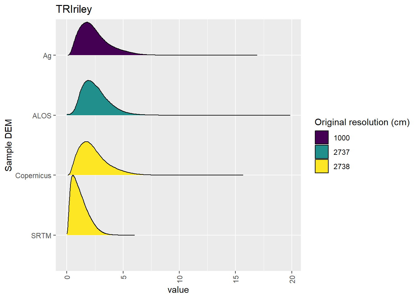
Figure 6.31: Distribution of TRIriley values in each DEM: Hambidge
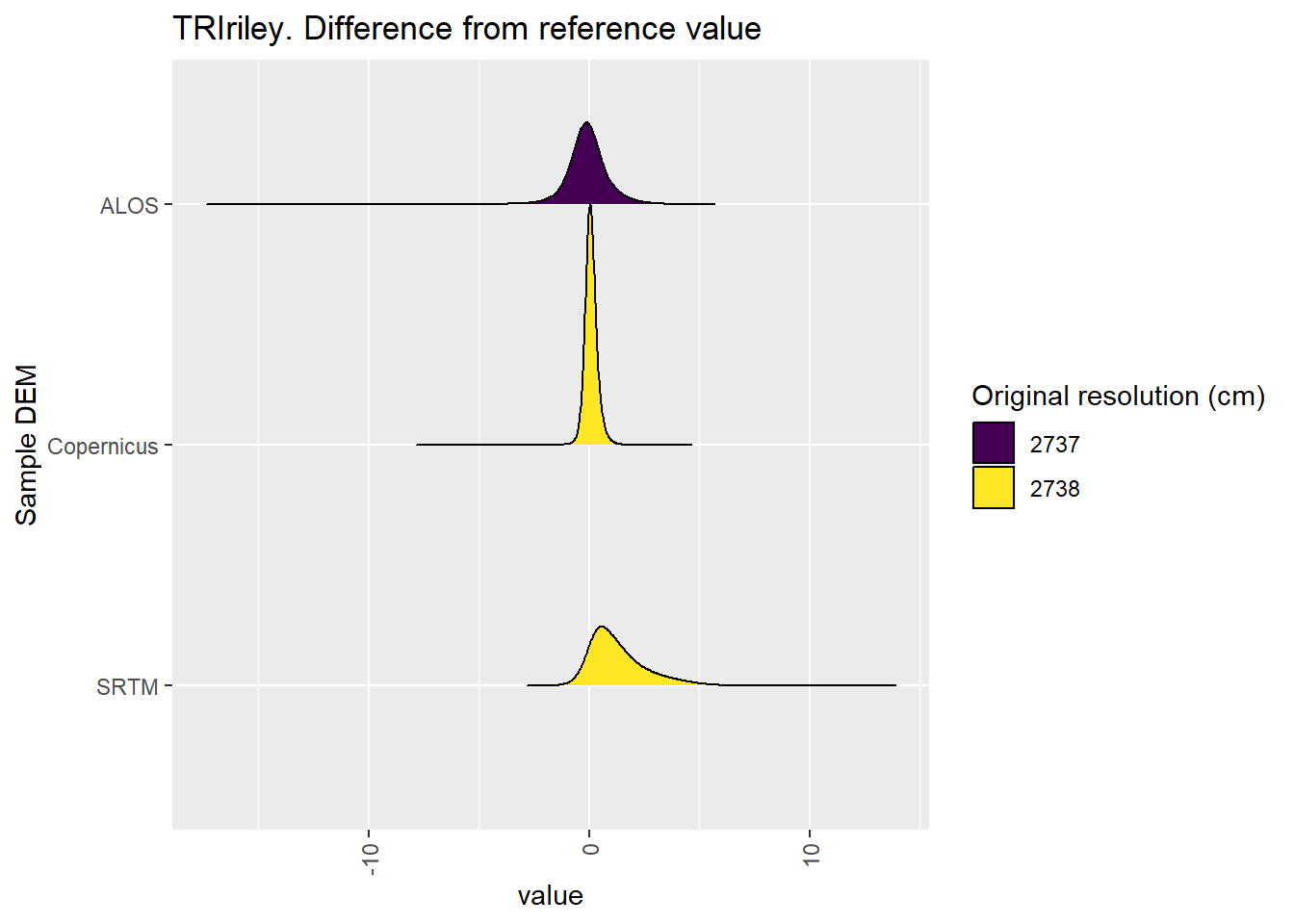
Figure 6.32: Distribution of difference between each DEM and reference for TRIriley values: Hambidge
6.1.9 TRIrmsd
Figure 6.33 shows rasters for TRIrmsd in the Hambidge area.
Table 6.34 shows boxplots for each decile of TRIrmsd, allowing a comparison of values within each DEM across different ranges of TRIrmsd. Deciles are based on the values in the reference DEM: Ag.
Figure 6.35 shows the a distribution of values for each sample DEM and window size.
Figure 6.36 shows the distribution of differences between the reference DEM and the other DEMs.
Figure 6.33: TRIrmsd raster for each DEM
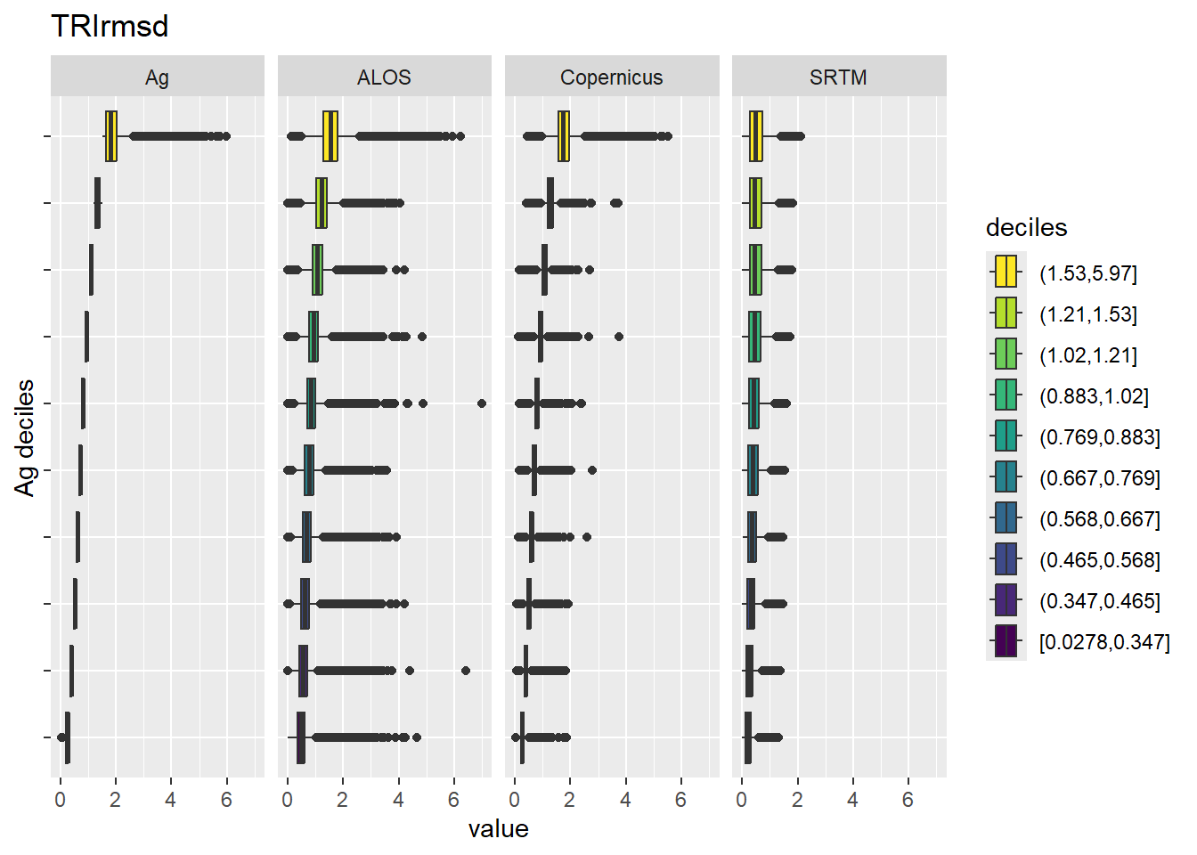
Figure 6.34: Range of values within deciles for each DEM. Deciles are taken from the reference DEM
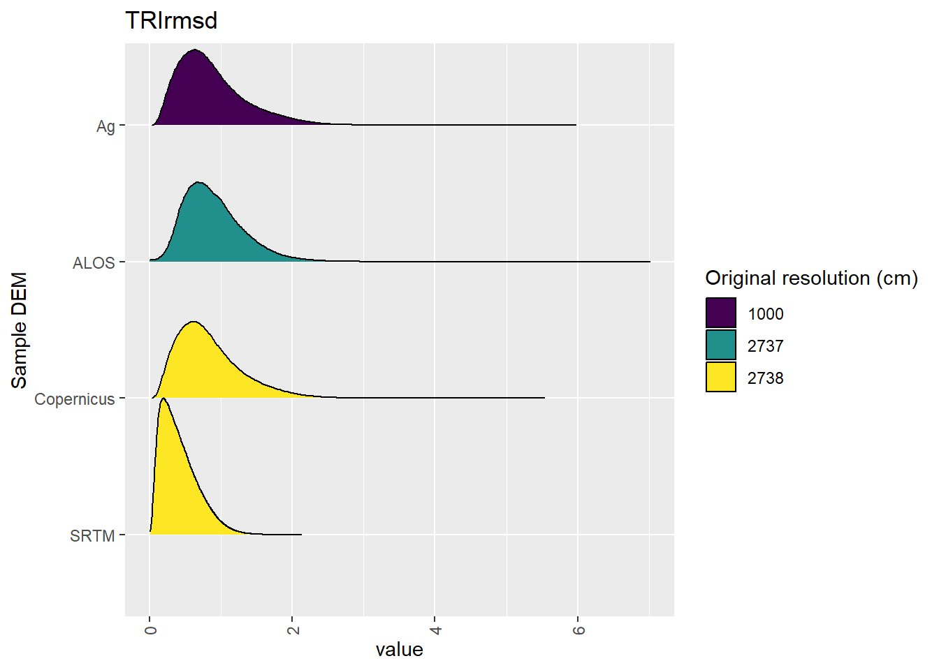
Figure 6.35: Distribution of TRIrmsd values in each DEM: Hambidge
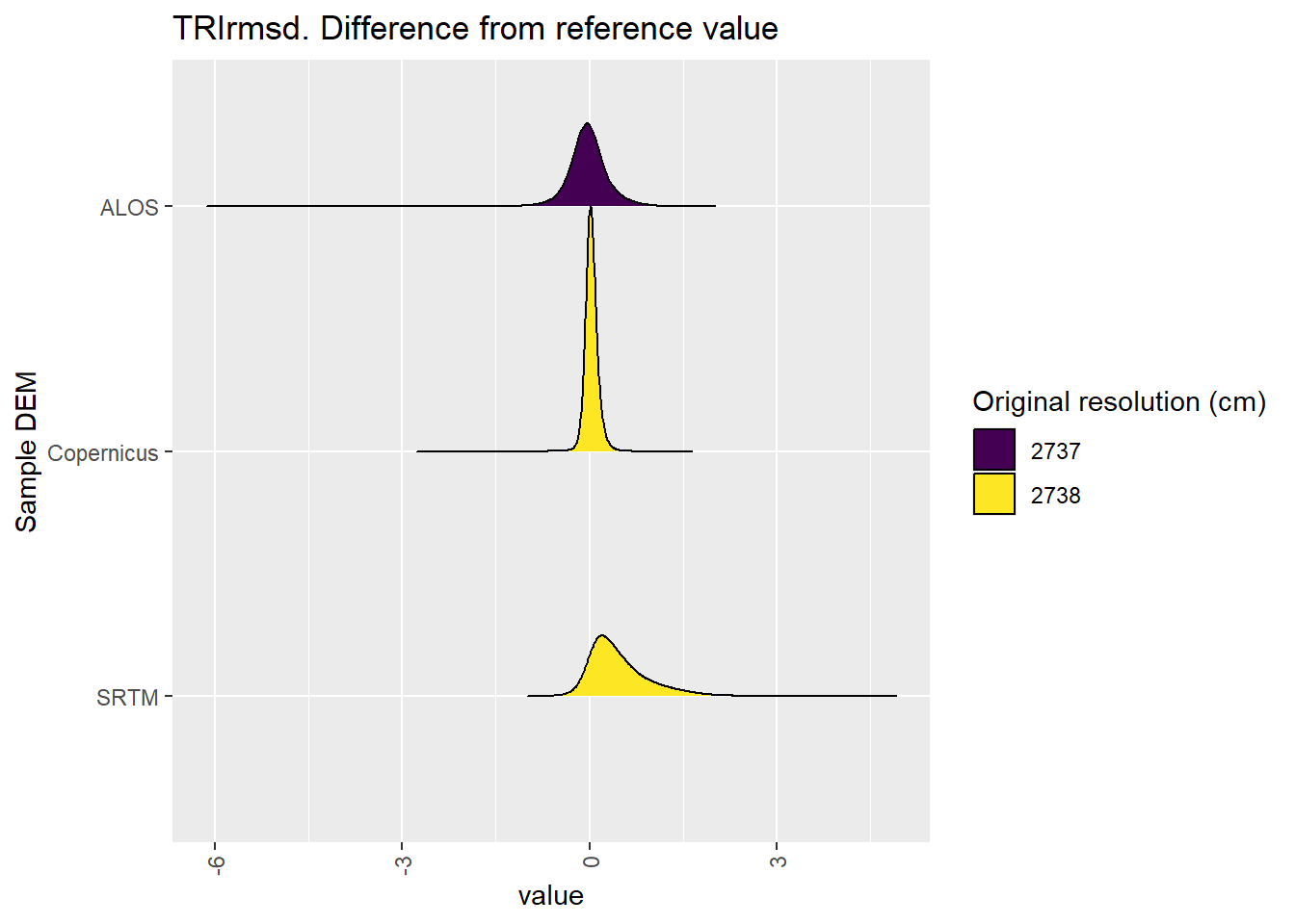
Figure 6.36: Distribution of difference between each DEM and reference for TRIrmsd values: Hambidge
6.1.10 roughness
Figure 6.37 shows rasters for roughness in the Hambidge area.
Table 6.38 shows boxplots for each decile of roughness, allowing a comparison of values within each DEM across different ranges of roughness. Deciles are based on the values in the reference DEM: Ag.
Figure 6.39 shows the a distribution of values for each sample DEM and window size.
Figure 6.40 shows the distribution of differences between the reference DEM and the other DEMs.
Figure 6.37: roughness raster for each DEM
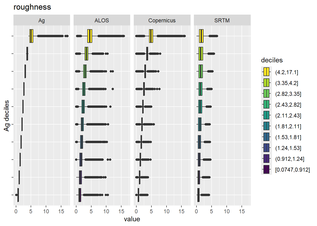
Figure 6.38: Range of values within deciles for each DEM. Deciles are taken from the reference DEM
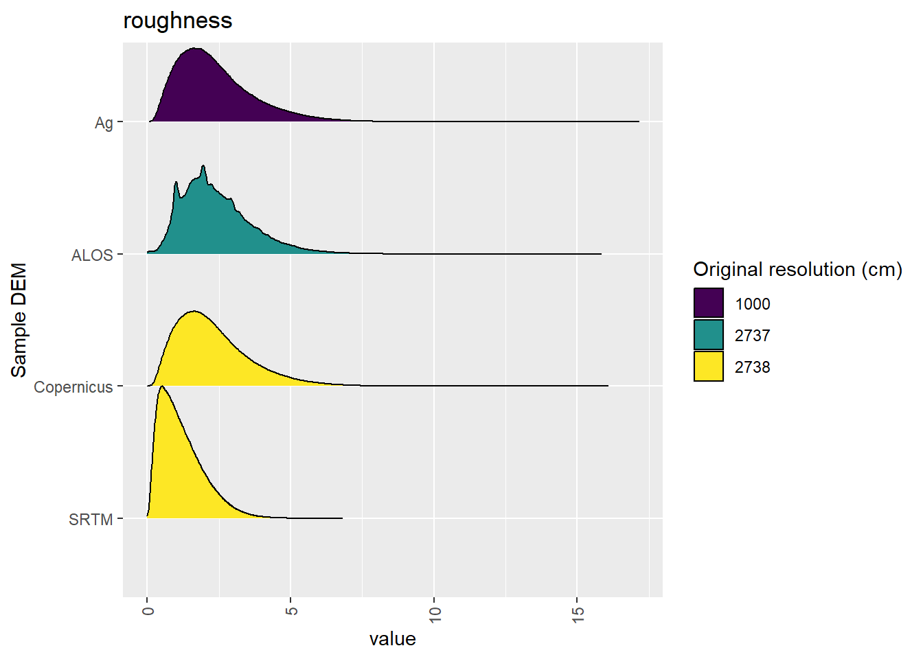
Figure 6.39: Distribution of roughness values in each DEM: Hambidge
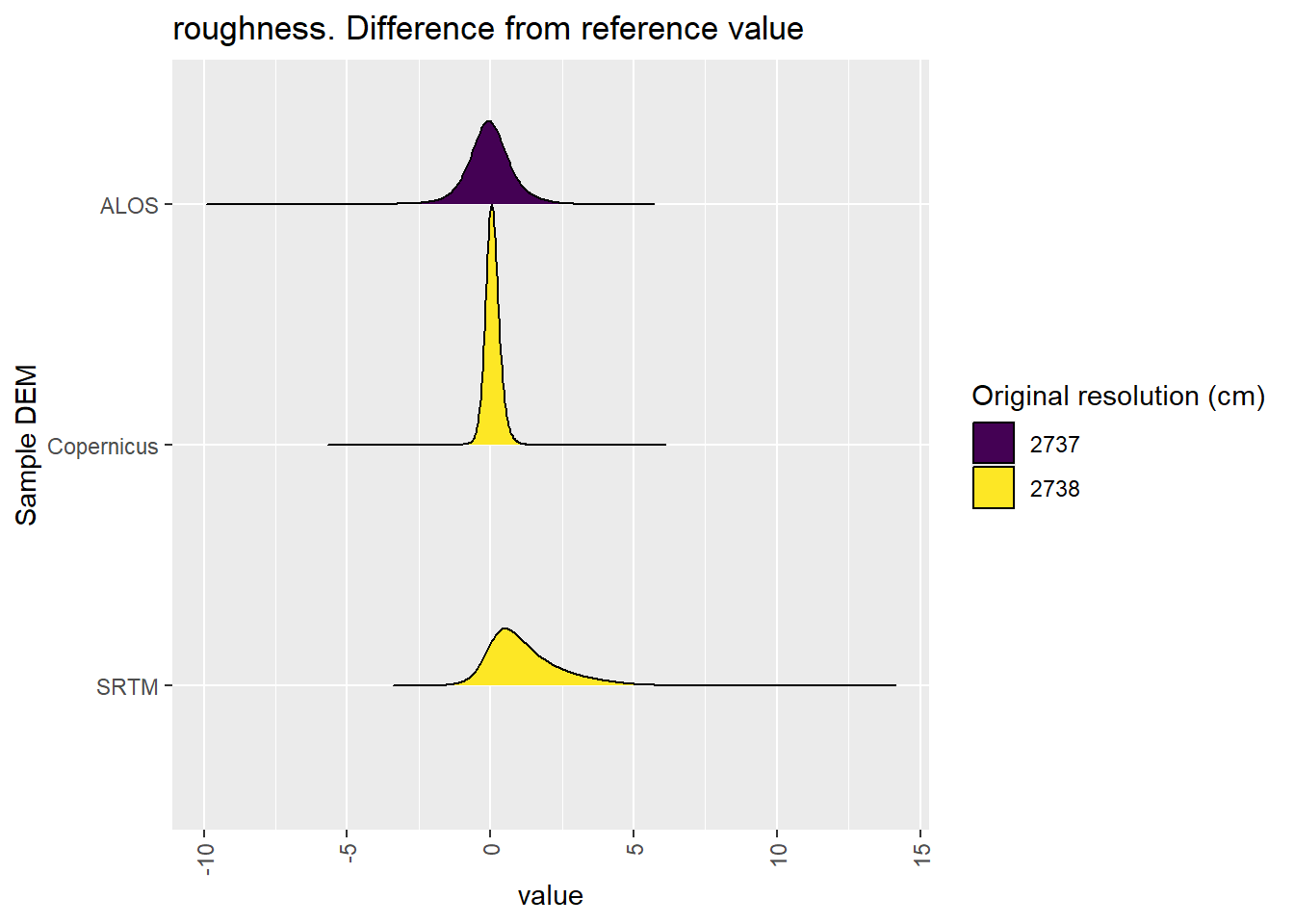
Figure 6.40: Distribution of difference between each DEM and reference for roughness values: Hambidge
6.2 Categorical
Table 6.1 shows the proportion of each DEM classifed to each landform element (also see Figure 6.42.
Figure 6.41 shows a landscape classification for each reprojected area.
| landform | Ag | ALOS | Copernicus | SRTM |
|---|---|---|---|---|
| canyon | 0.0093786 | 0.0168795 | 0.0085566 | 0.00242 |
| midslope drainage | 0.0096920 | 0.0136367 | 0.0084797 | 0.00119 |
| upland drainage | 0.0000077 | 0.0000048 | 0.0000038 | |
| u-shaped valley | 0.0539199 | 0.0611180 | 0.0548226 | 0.02408 |
| plains | 0.8188237 | 0.8018144 | 0.8249066 | 0.94202 |
| open slopes | 0.0081162 | 0.0046609 | 0.0060934 | |
| upper slopes | 0.0767188 | 0.0733068 | 0.0764688 | 0.02725 |
| local ridges | 0.0000115 | 0.0000163 | 0.0000067 | |
| midslopes ridges | 0.0094651 | 0.0137819 | 0.0083181 | 0.00061 |
| mountain tops | 0.0138665 | 0.0147808 | 0.0123436 | 0.00243 |
Figure 6.41: Categorical representation of Hambidge
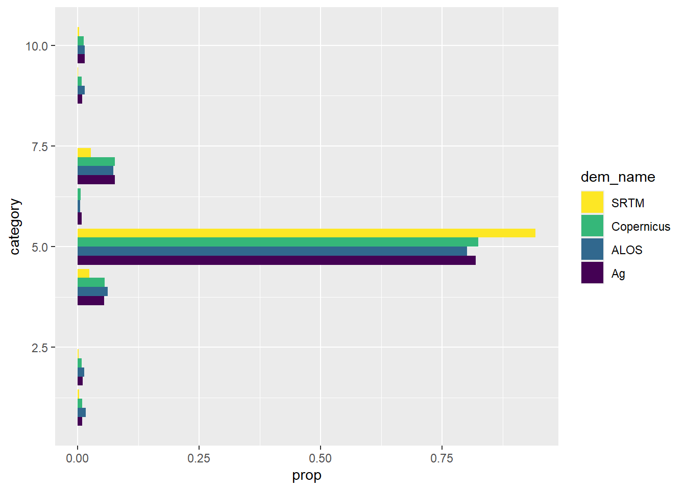
Figure 6.42: Proportion of categorised Hambidge area in each of several classification classes