8 Deep Creek
8.1 Continuous
8.1.1 elev
Figure 8.1 shows rasters for elev in the Deep Creek area.
Table 8.2 shows boxplots for each decile of elev, allowing a comparison of values within each DEM across different ranges of elev. Deciles are based on the values in the reference DEM: Ag.
Figure 8.3 shows the a distribution of values for each sample DEM and window size.
Figure 8.4 shows the distribution of differences between the reference DEM and the other DEMs.
Figure 8.1: elev raster for each DEM
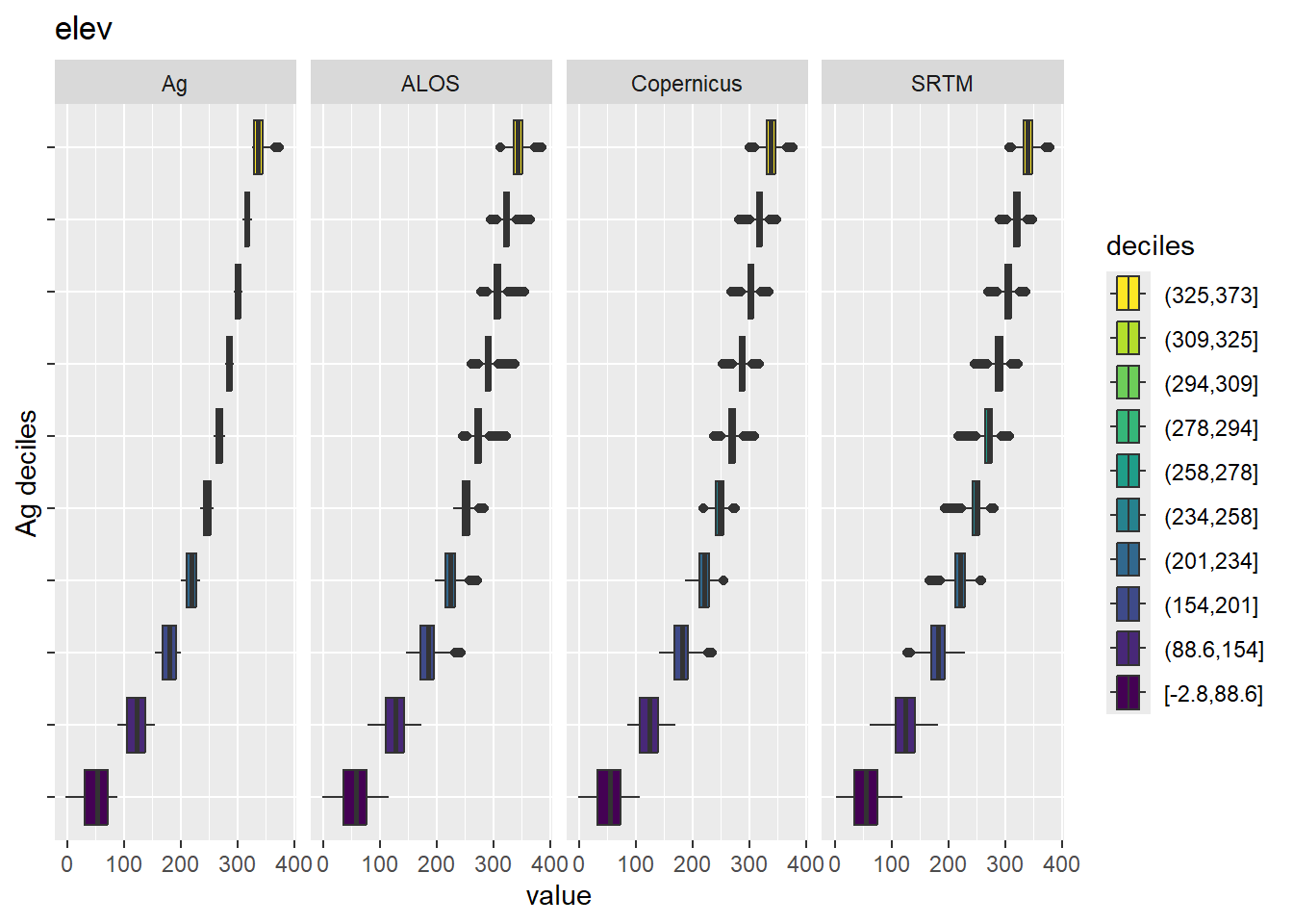
Figure 8.2: Range of values within deciles for each DEM. Deciles are taken from the reference DEM
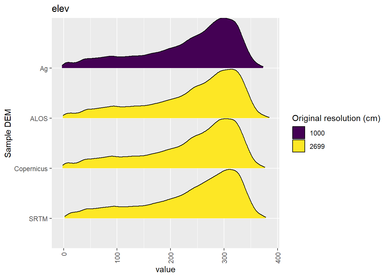
Figure 8.3: Distribution of elev values in each DEM: Deep Creek
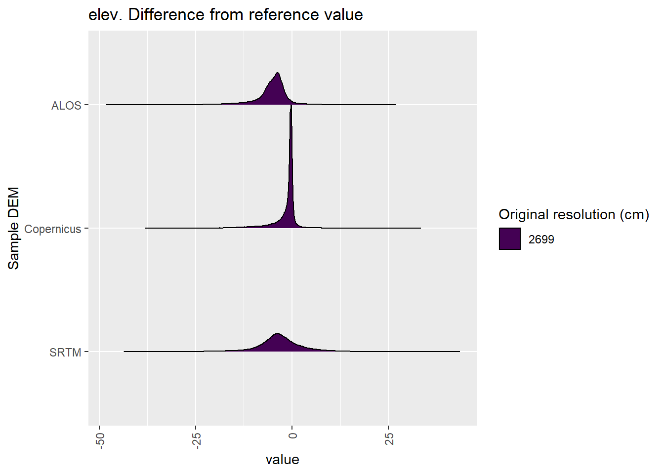
Figure 8.4: Distribution of difference between each DEM and reference for elev values: Deep Creek
8.1.2 qslope
Figure 8.5 shows rasters for qslope in the Deep Creek area.
Table 8.6 shows boxplots for each decile of qslope, allowing a comparison of values within each DEM across different ranges of qslope. Deciles are based on the values in the reference DEM: Ag.
Figure 8.7 shows the a distribution of values for each sample DEM and window size.
Figure 8.8 shows the distribution of differences between the reference DEM and the other DEMs.
Figure 8.5: qslope raster for each DEM
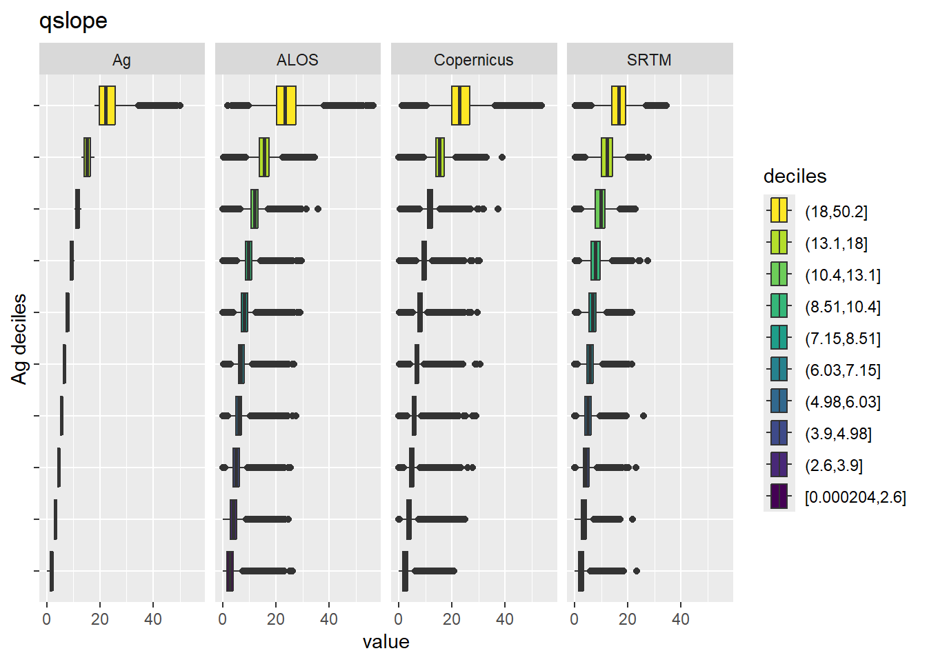
Figure 8.6: Range of values within deciles for each DEM. Deciles are taken from the reference DEM
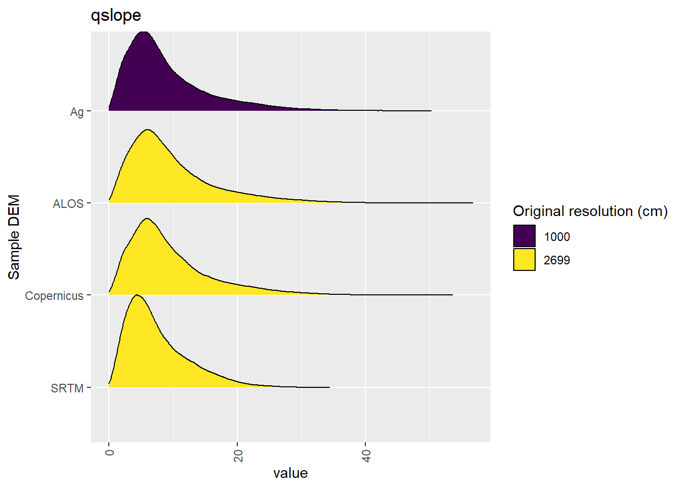
Figure 8.7: Distribution of qslope values in each DEM: Deep Creek
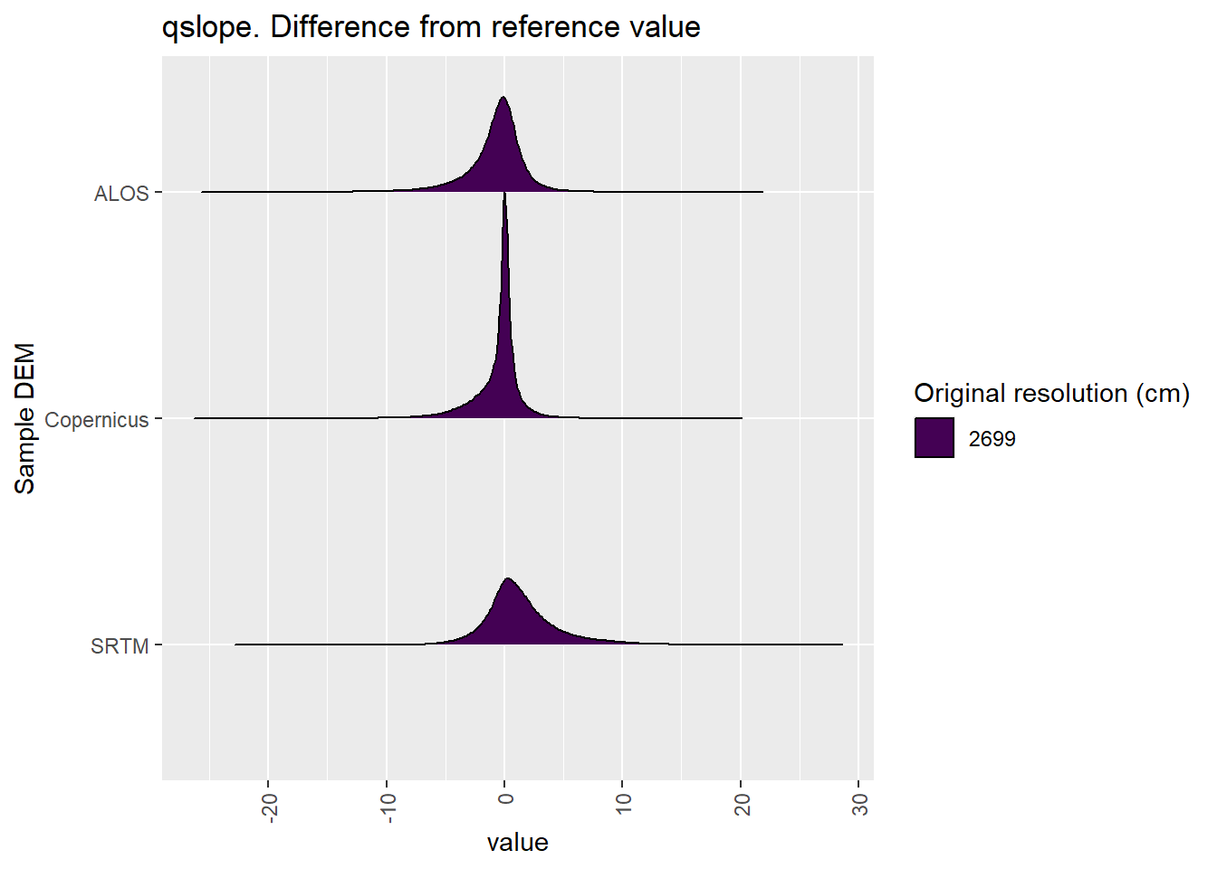
Figure 8.8: Distribution of difference between each DEM and reference for qslope values: Deep Creek
8.1.3 qaspect
Figure 8.9 shows rasters for qaspect in the Deep Creek area.
Table 8.10 shows boxplots for each decile of qaspect, allowing a comparison of values within each DEM across different ranges of qaspect. Deciles are based on the values in the reference DEM: Ag.
Figure 8.11 shows the a distribution of values for each sample DEM and window size.
Figure 8.12 shows the distribution of differences between the reference DEM and the other DEMs.
Figure 8.9: qaspect raster for each DEM
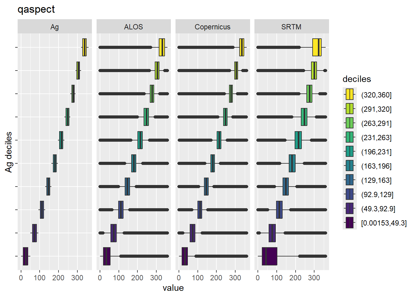
Figure 8.10: Range of values within deciles for each DEM. Deciles are taken from the reference DEM
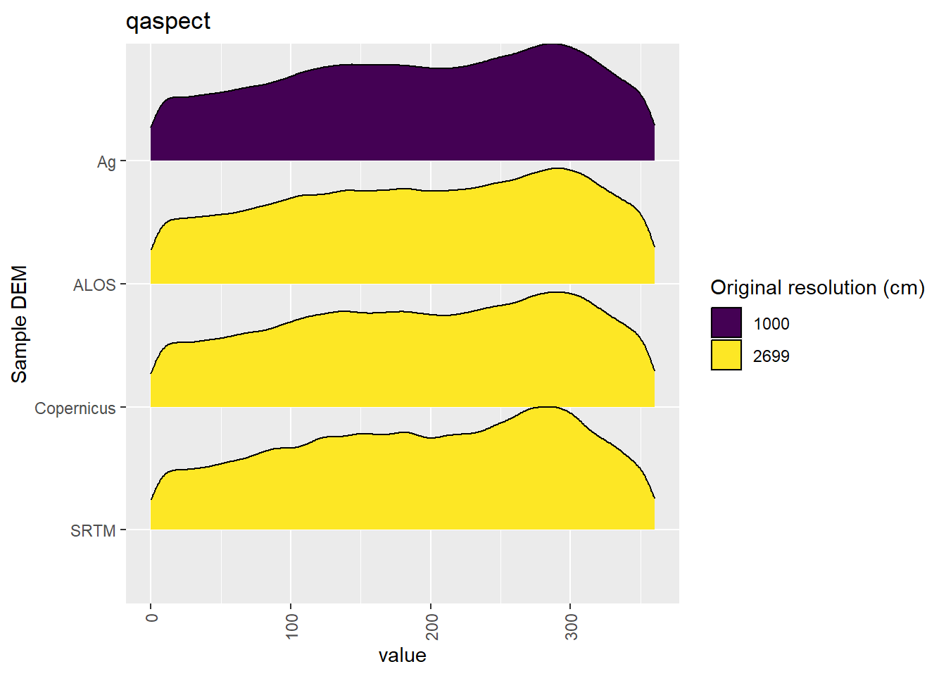
Figure 8.11: Distribution of qaspect values in each DEM: Deep Creek
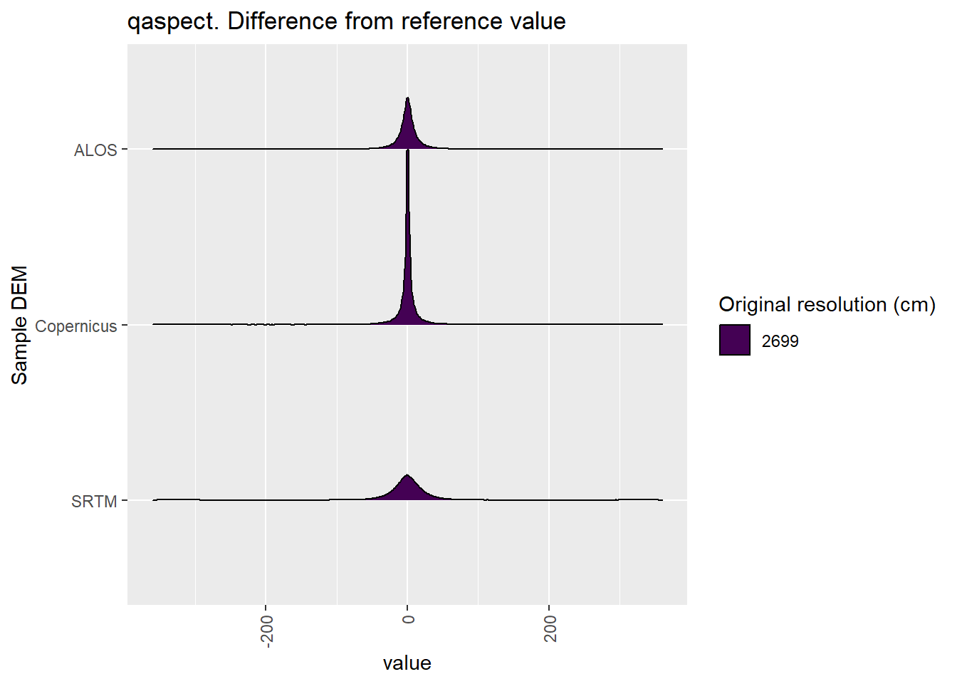
Figure 8.12: Distribution of difference between each DEM and reference for qaspect values: Deep Creek
8.1.4 qeastness
Figure 8.13 shows rasters for qeastness in the Deep Creek area.
Table 8.14 shows boxplots for each decile of qeastness, allowing a comparison of values within each DEM across different ranges of qeastness. Deciles are based on the values in the reference DEM: Ag.
Figure 8.15 shows the a distribution of values for each sample DEM and window size.
Figure 8.16 shows the distribution of differences between the reference DEM and the other DEMs.
Figure 8.13: qeastness raster for each DEM
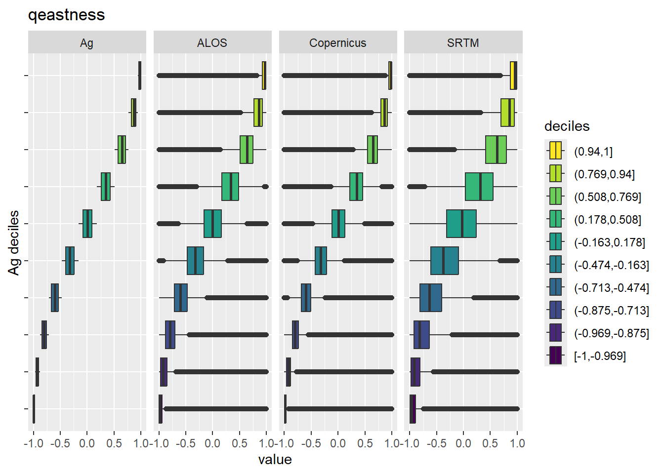
Figure 8.14: Range of values within deciles for each DEM. Deciles are taken from the reference DEM
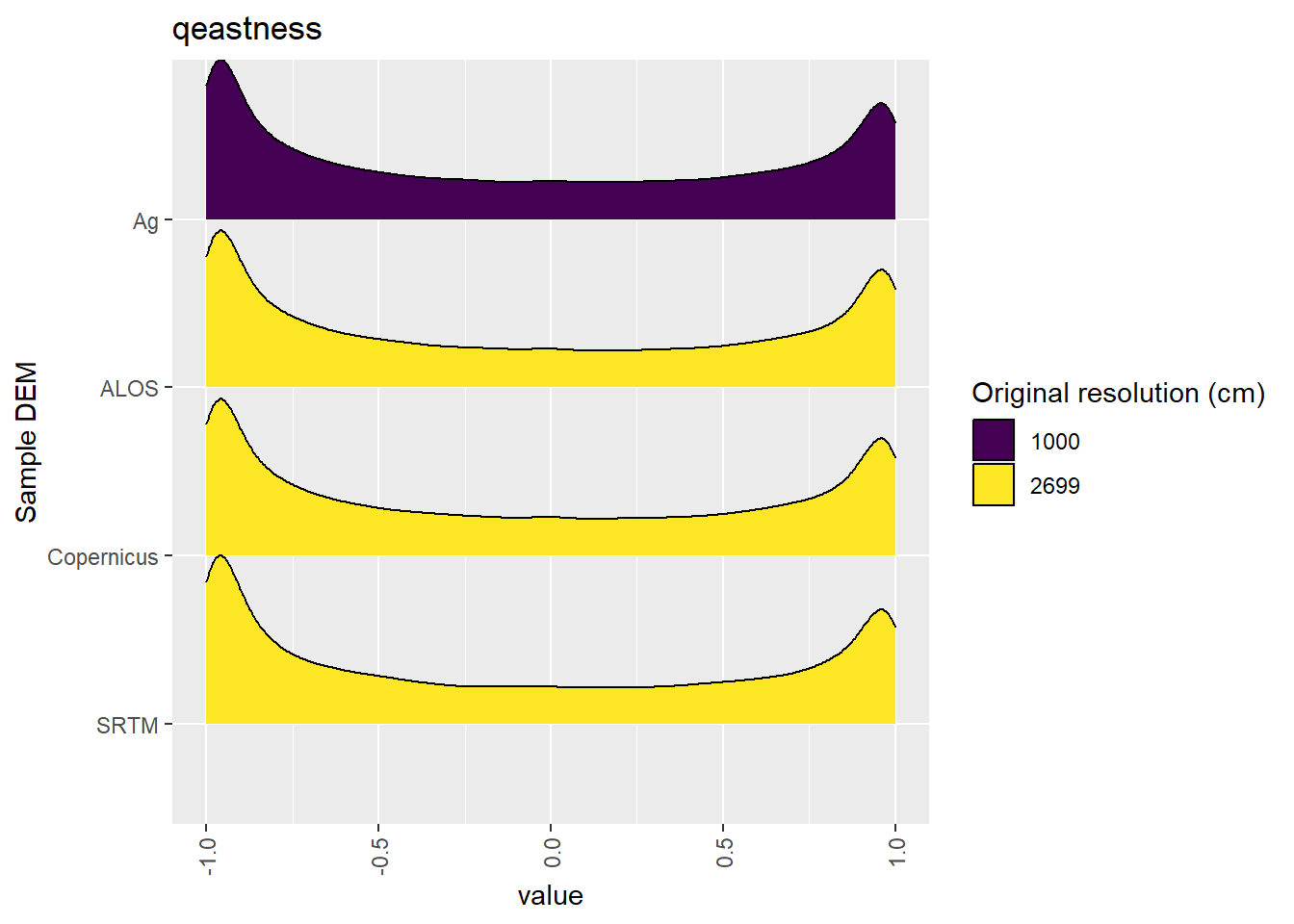
Figure 8.15: Distribution of qeastness values in each DEM: Deep Creek
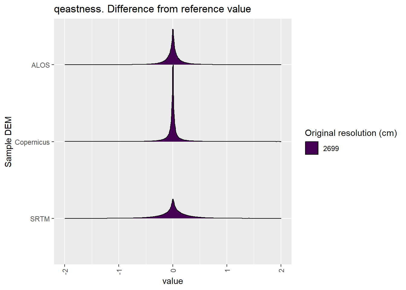
Figure 8.16: Distribution of difference between each DEM and reference for qeastness values: Deep Creek
8.1.5 qnorthness
Figure 8.17 shows rasters for qnorthness in the Deep Creek area.
Table 8.18 shows boxplots for each decile of qnorthness, allowing a comparison of values within each DEM across different ranges of qnorthness. Deciles are based on the values in the reference DEM: Ag.
Figure 8.19 shows the a distribution of values for each sample DEM and window size.
Figure 8.20 shows the distribution of differences between the reference DEM and the other DEMs.
Figure 8.17: qnorthness raster for each DEM
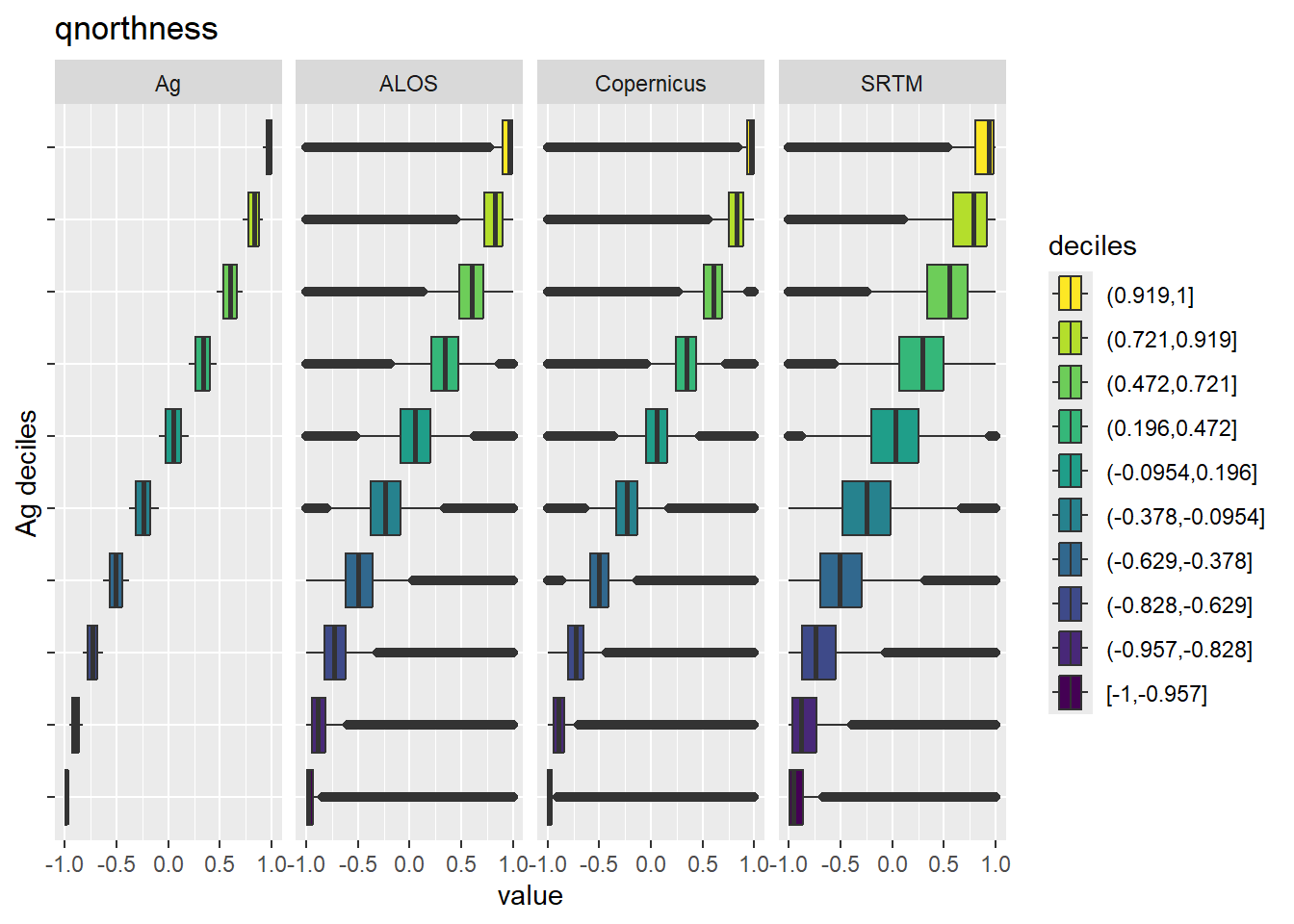
Figure 8.18: Range of values within deciles for each DEM. Deciles are taken from the reference DEM
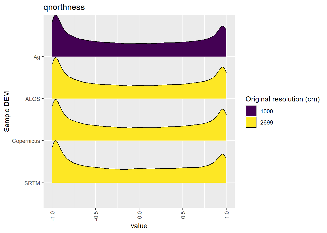
Figure 8.19: Distribution of qnorthness values in each DEM: Deep Creek
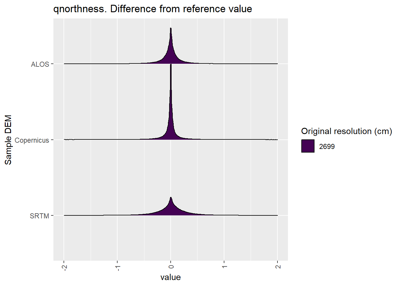
Figure 8.20: Distribution of difference between each DEM and reference for qnorthness values: Deep Creek
8.1.6 TPI
Figure 8.21 shows rasters for TPI in the Deep Creek area.
Table 8.22 shows boxplots for each decile of TPI, allowing a comparison of values within each DEM across different ranges of TPI. Deciles are based on the values in the reference DEM: Ag.
Figure 8.23 shows the a distribution of values for each sample DEM and window size.
Figure 8.24 shows the distribution of differences between the reference DEM and the other DEMs.
Figure 8.21: TPI raster for each DEM
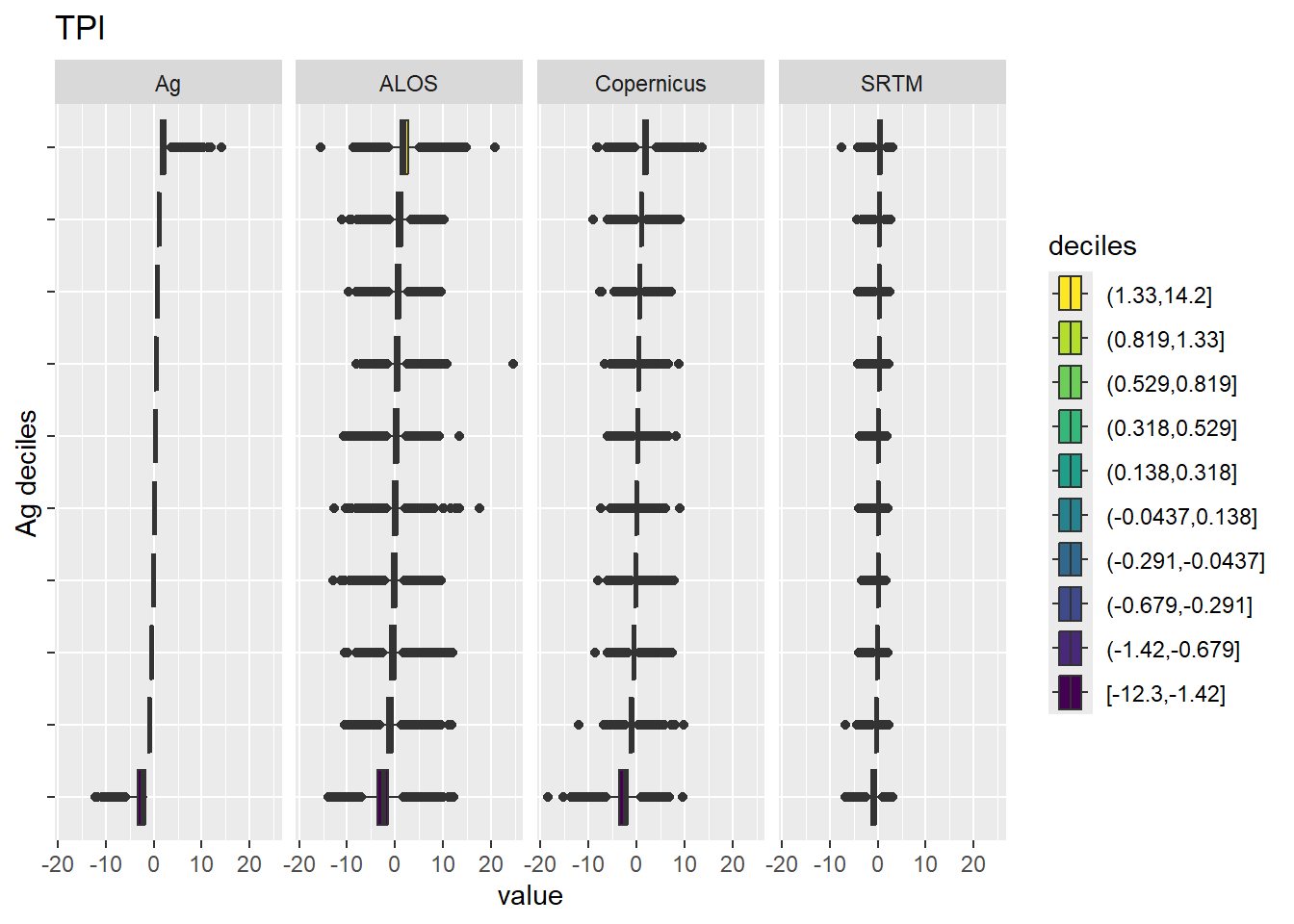
Figure 8.22: Range of values within deciles for each DEM. Deciles are taken from the reference DEM
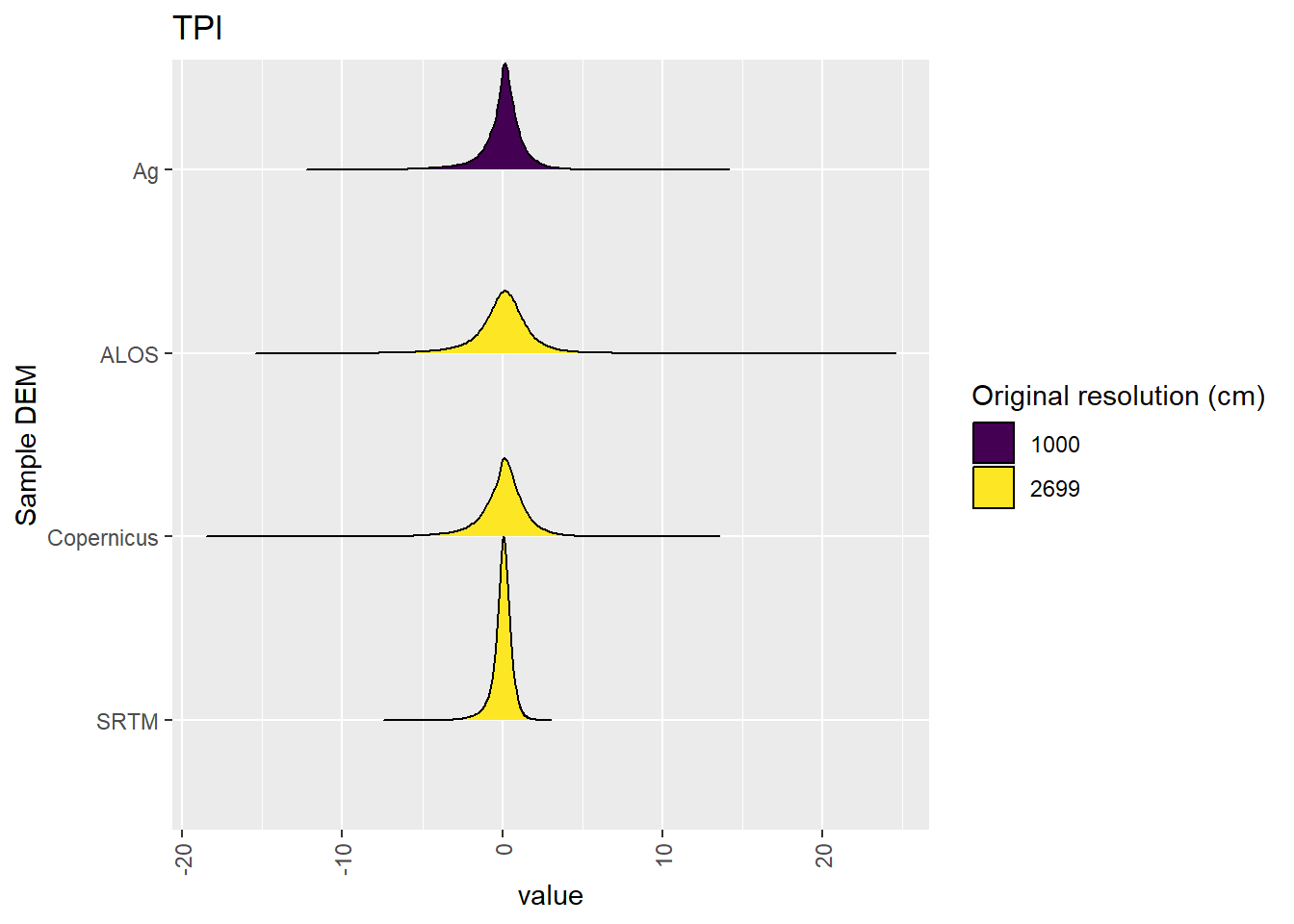
Figure 8.23: Distribution of TPI values in each DEM: Deep Creek
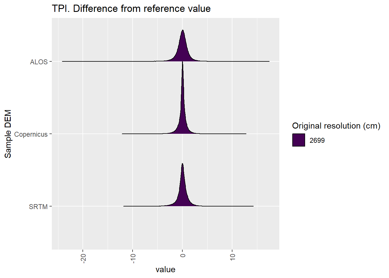
Figure 8.24: Distribution of difference between each DEM and reference for TPI values: Deep Creek
8.1.7 TRI
Figure 8.25 shows rasters for TRI in the Deep Creek area.
Table 8.26 shows boxplots for each decile of TRI, allowing a comparison of values within each DEM across different ranges of TRI. Deciles are based on the values in the reference DEM: Ag.
Figure 8.27 shows the a distribution of values for each sample DEM and window size.
Figure 8.28 shows the distribution of differences between the reference DEM and the other DEMs.
Figure 8.25: TRI raster for each DEM
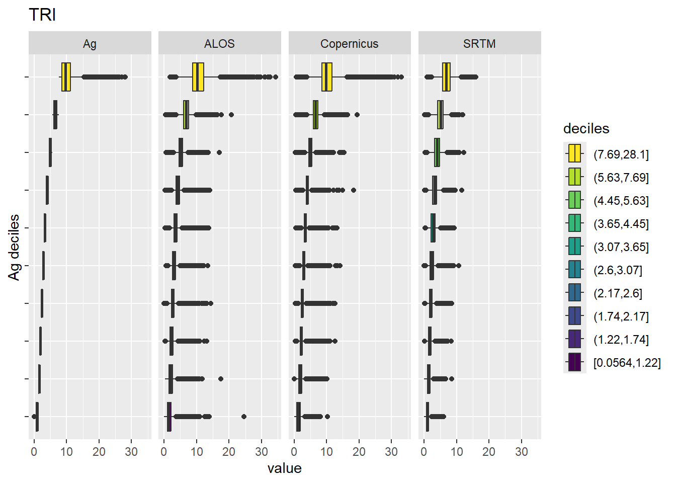
Figure 8.26: Range of values within deciles for each DEM. Deciles are taken from the reference DEM
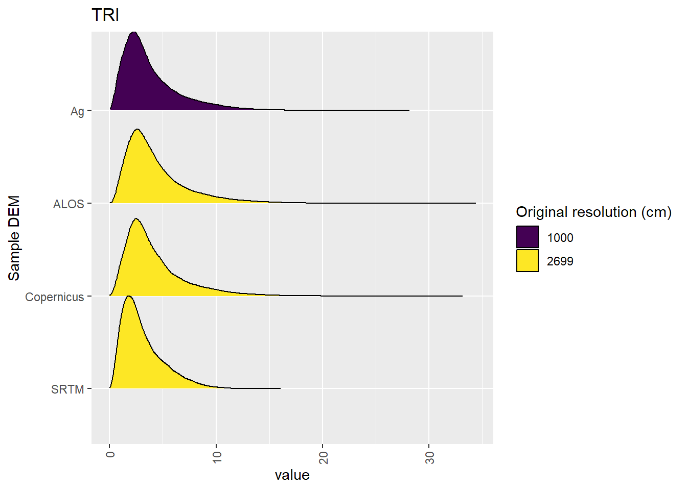
Figure 8.27: Distribution of TRI values in each DEM: Deep Creek
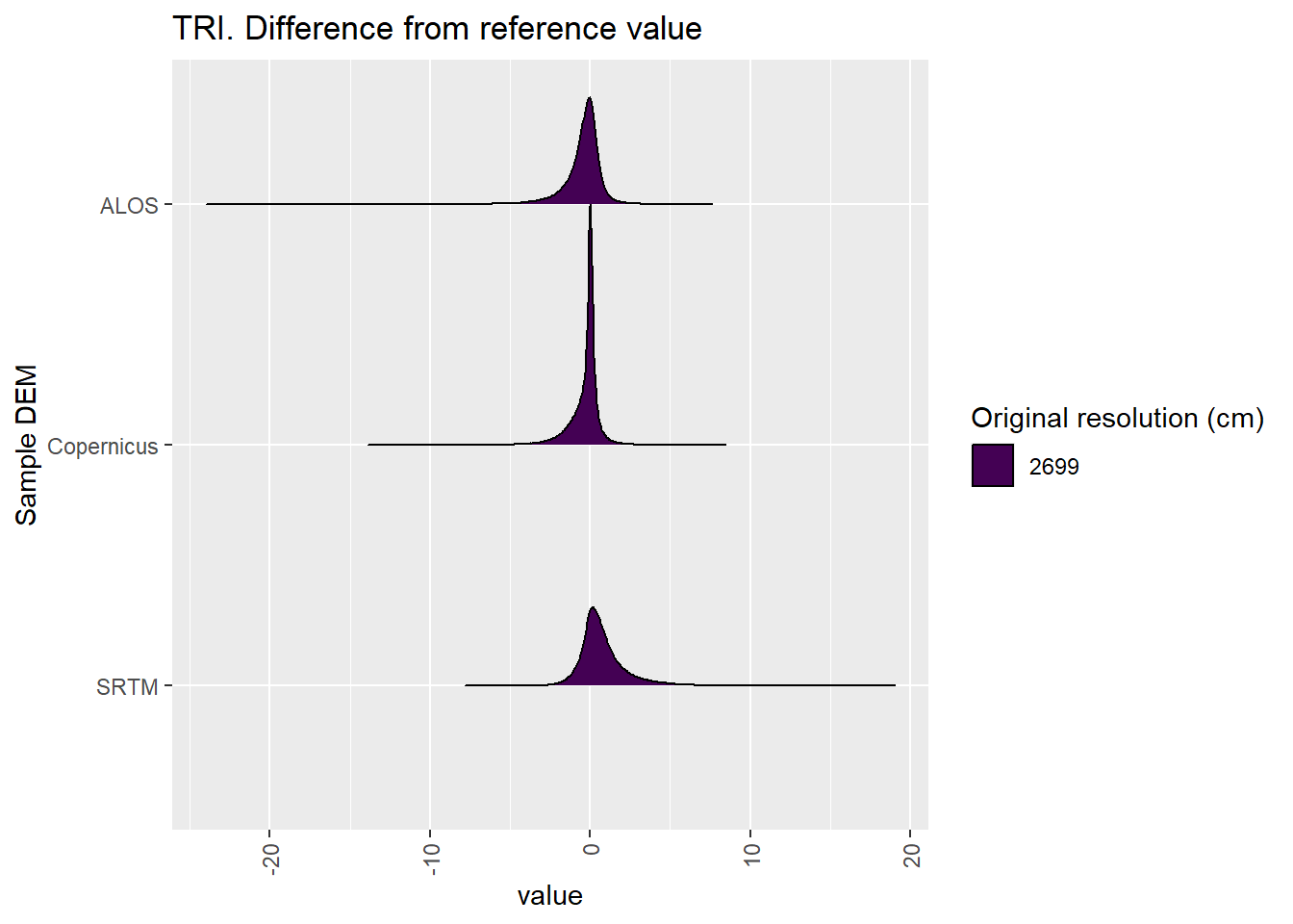
Figure 8.28: Distribution of difference between each DEM and reference for TRI values: Deep Creek
8.1.8 TRIriley
Figure 8.29 shows rasters for TRIriley in the Deep Creek area.
Table 8.30 shows boxplots for each decile of TRIriley, allowing a comparison of values within each DEM across different ranges of TRIriley. Deciles are based on the values in the reference DEM: Ag.
Figure 8.31 shows the a distribution of values for each sample DEM and window size.
Figure 8.32 shows the distribution of differences between the reference DEM and the other DEMs.
Figure 8.29: TRIriley raster for each DEM
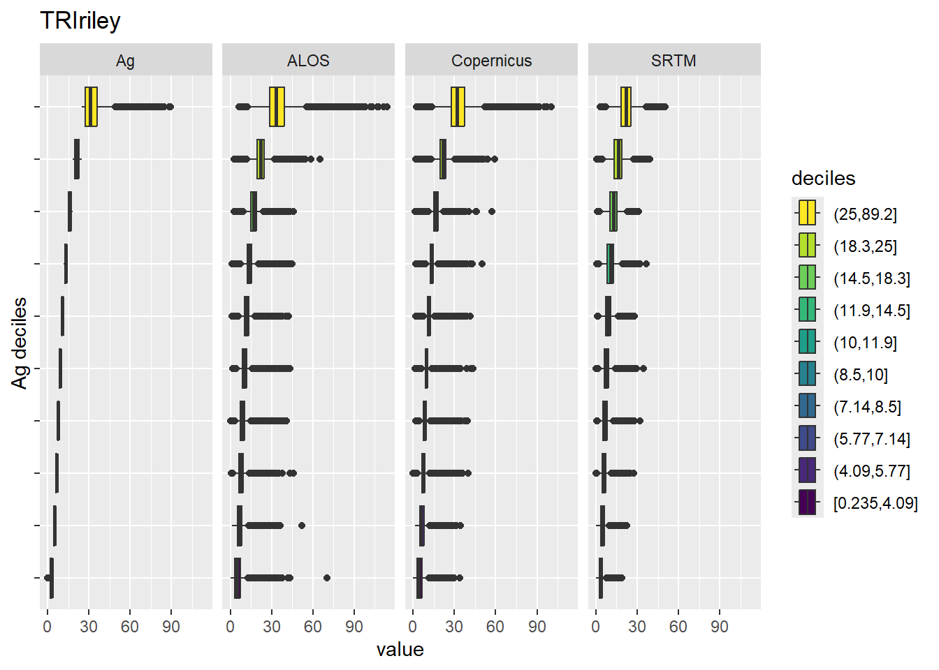
Figure 8.30: Range of values within deciles for each DEM. Deciles are taken from the reference DEM

Figure 8.31: Distribution of TRIriley values in each DEM: Deep Creek
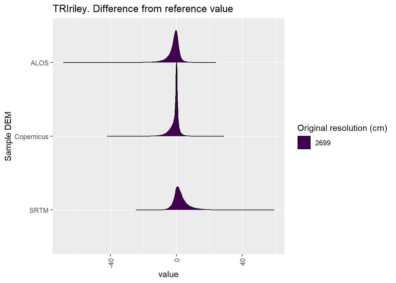
Figure 8.32: Distribution of difference between each DEM and reference for TRIriley values: Deep Creek
8.1.9 TRIrmsd
Figure 8.33 shows rasters for TRIrmsd in the Deep Creek area.
Table 8.34 shows boxplots for each decile of TRIrmsd, allowing a comparison of values within each DEM across different ranges of TRIrmsd. Deciles are based on the values in the reference DEM: Ag.
Figure 8.35 shows the a distribution of values for each sample DEM and window size.
Figure 8.36 shows the distribution of differences between the reference DEM and the other DEMs.
Figure 8.33: TRIrmsd raster for each DEM
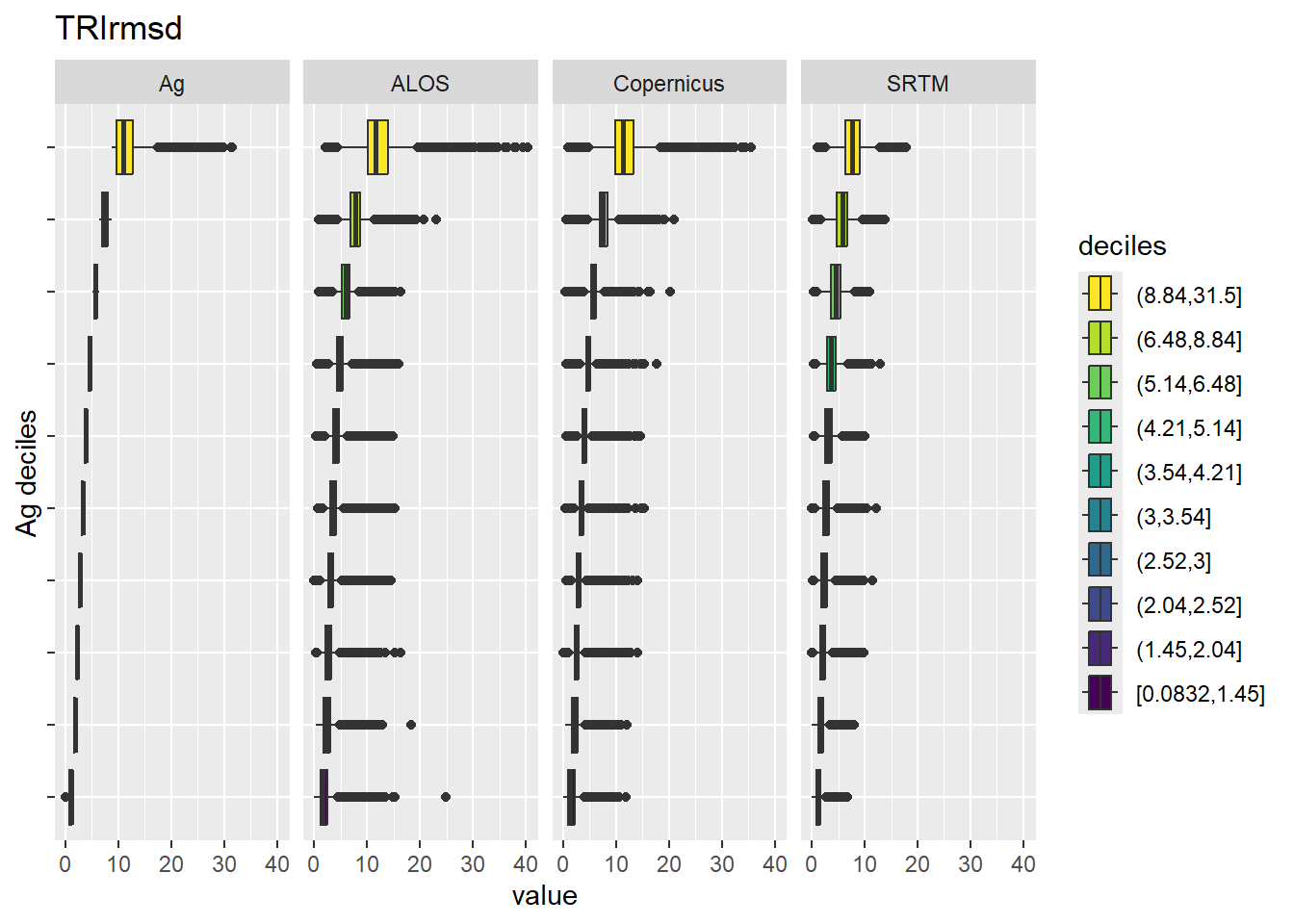
Figure 8.34: Range of values within deciles for each DEM. Deciles are taken from the reference DEM
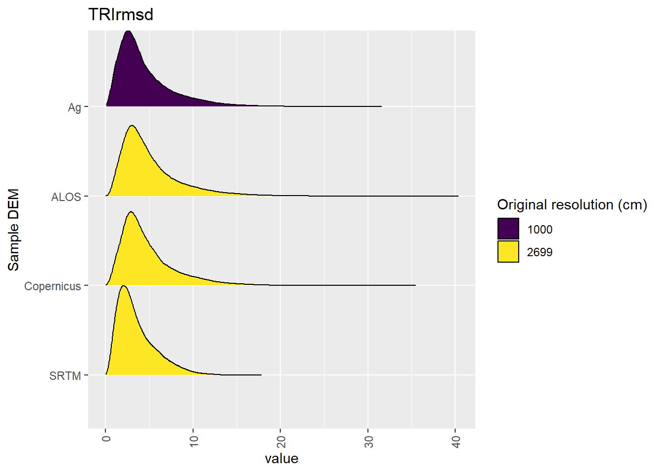
Figure 8.35: Distribution of TRIrmsd values in each DEM: Deep Creek
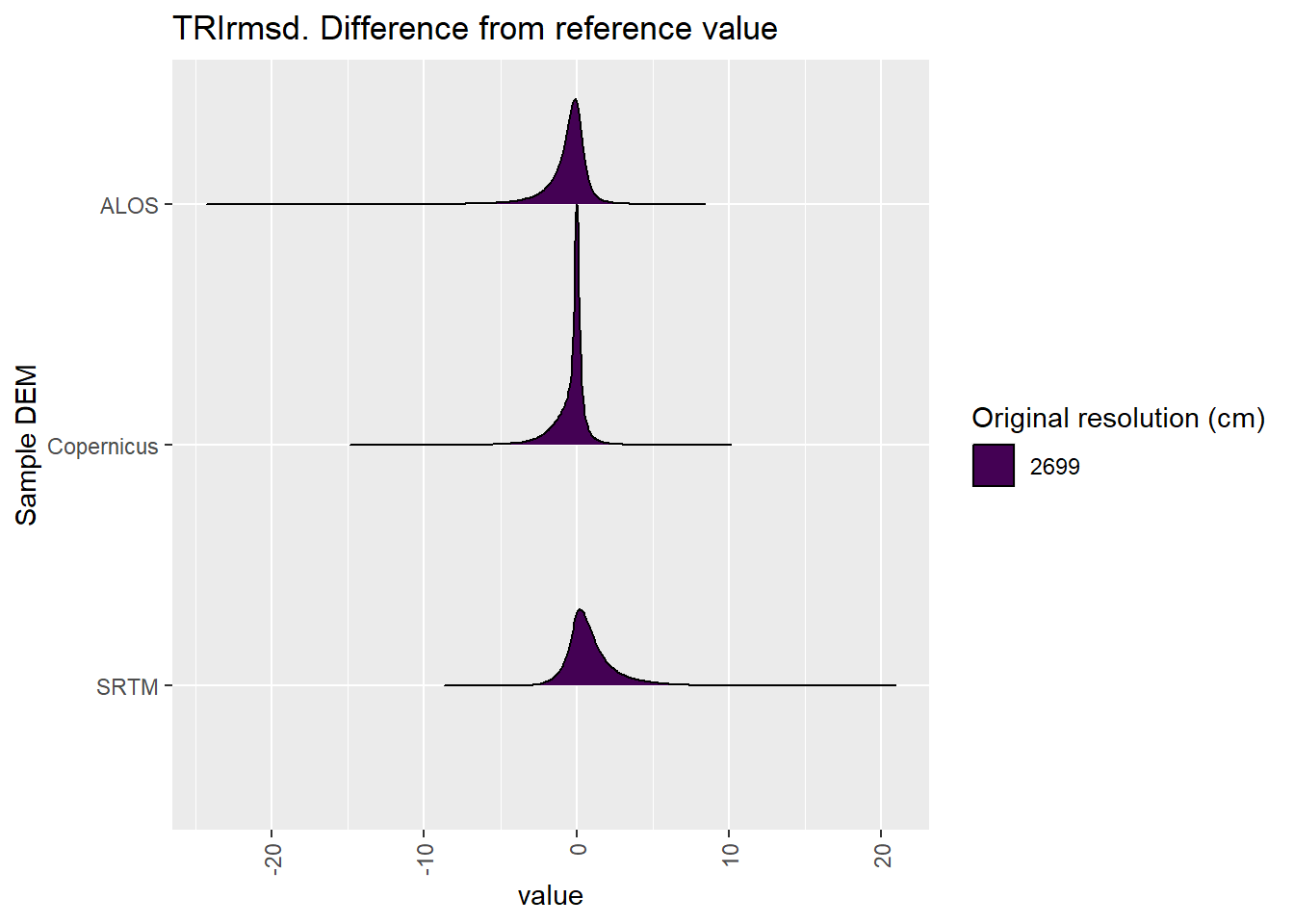
Figure 8.36: Distribution of difference between each DEM and reference for TRIrmsd values: Deep Creek
8.1.10 roughness
Figure 8.37 shows rasters for roughness in the Deep Creek area.
Table 8.38 shows boxplots for each decile of roughness, allowing a comparison of values within each DEM across different ranges of roughness. Deciles are based on the values in the reference DEM: Ag.
Figure 8.39 shows the a distribution of values for each sample DEM and window size.
Figure 8.40 shows the distribution of differences between the reference DEM and the other DEMs.
Figure 8.37: roughness raster for each DEM
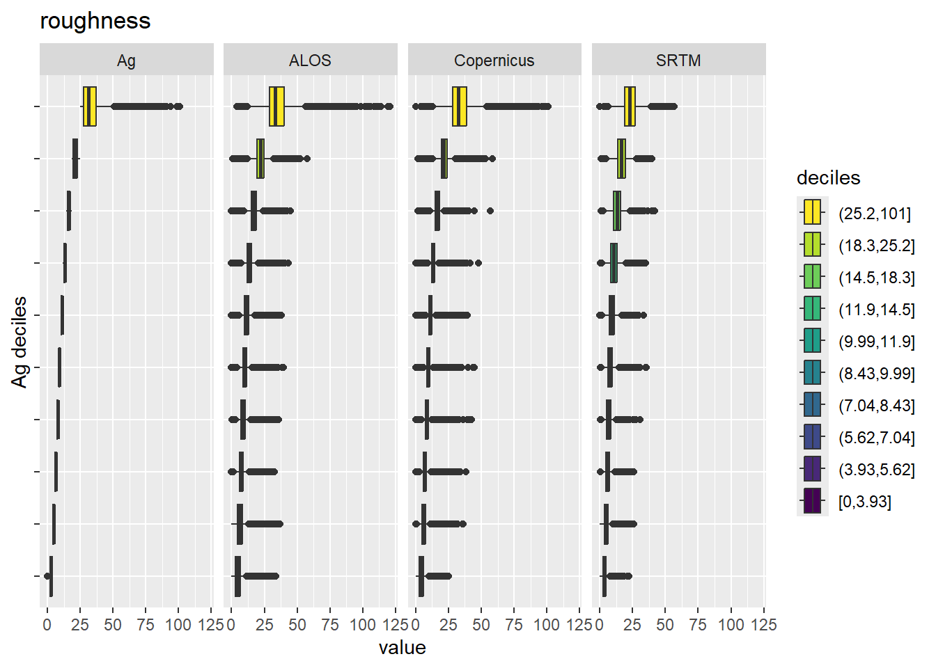
Figure 8.38: Range of values within deciles for each DEM. Deciles are taken from the reference DEM
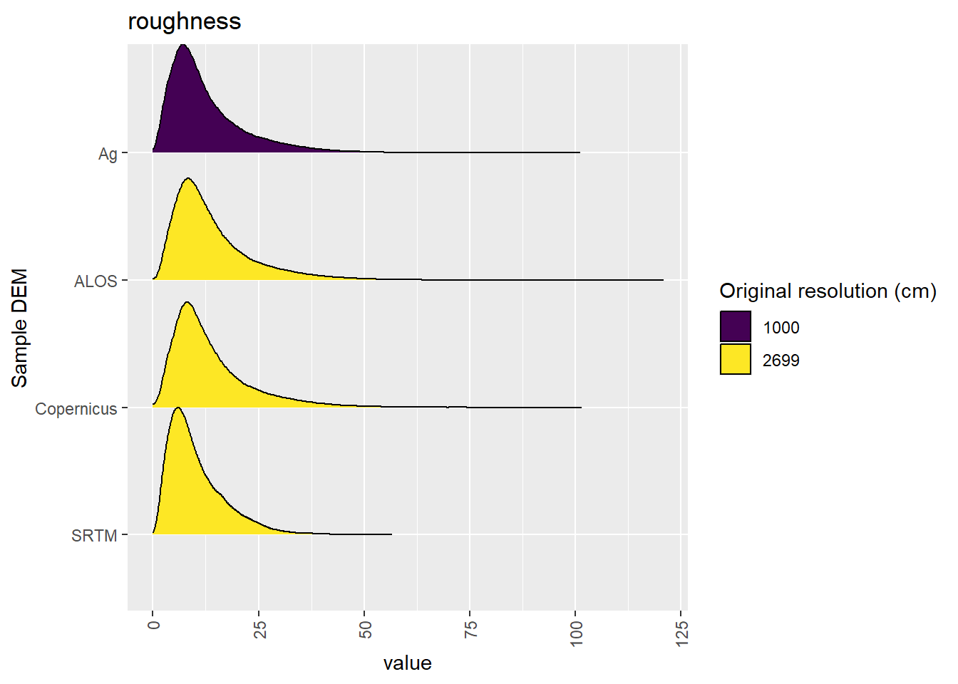
Figure 8.39: Distribution of roughness values in each DEM: Deep Creek
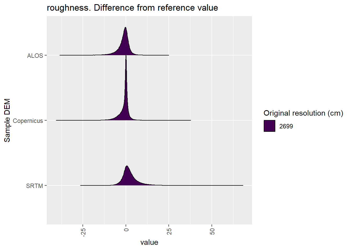
Figure 8.40: Distribution of difference between each DEM and reference for roughness values: Deep Creek
8.2 Categorical
Table 8.1 shows the proportion of each DEM classifed to each landform element (also see Figure 8.42.
Figure 8.41 shows a landscape classification for each reprojected area.
| landform | Ag | ALOS | Copernicus | SRTM |
|---|---|---|---|---|
| canyon | 0.0055157 | 0.0078897 | 0.0065220 | 0.001670 |
| midslope drainage | 0.0012373 | 0.0044499 | 0.0025417 | 0.000097 |
| upland drainage | 0.0000075 | 0.0000075 | ||
| u-shaped valley | 0.0475621 | 0.0514827 | 0.0506442 | 0.026379 |
| plains | 0.2519911 | 0.1891750 | 0.1953504 | 0.328496 |
| open slopes | 0.6567272 | 0.6939211 | 0.6959560 | 0.618803 |
| upper slopes | 0.0320882 | 0.0399966 | 0.0397282 | 0.022216 |
| midslopes ridges | 0.0013081 | 0.0050424 | 0.0029219 | 0.000224 |
| mountain tops | 0.0035666 | 0.0080351 | 0.0063245 | 0.002117 |
| local ridges | 0.0000037 | 0.0000037 |
Figure 8.41: Categorical representation of Deep Creek
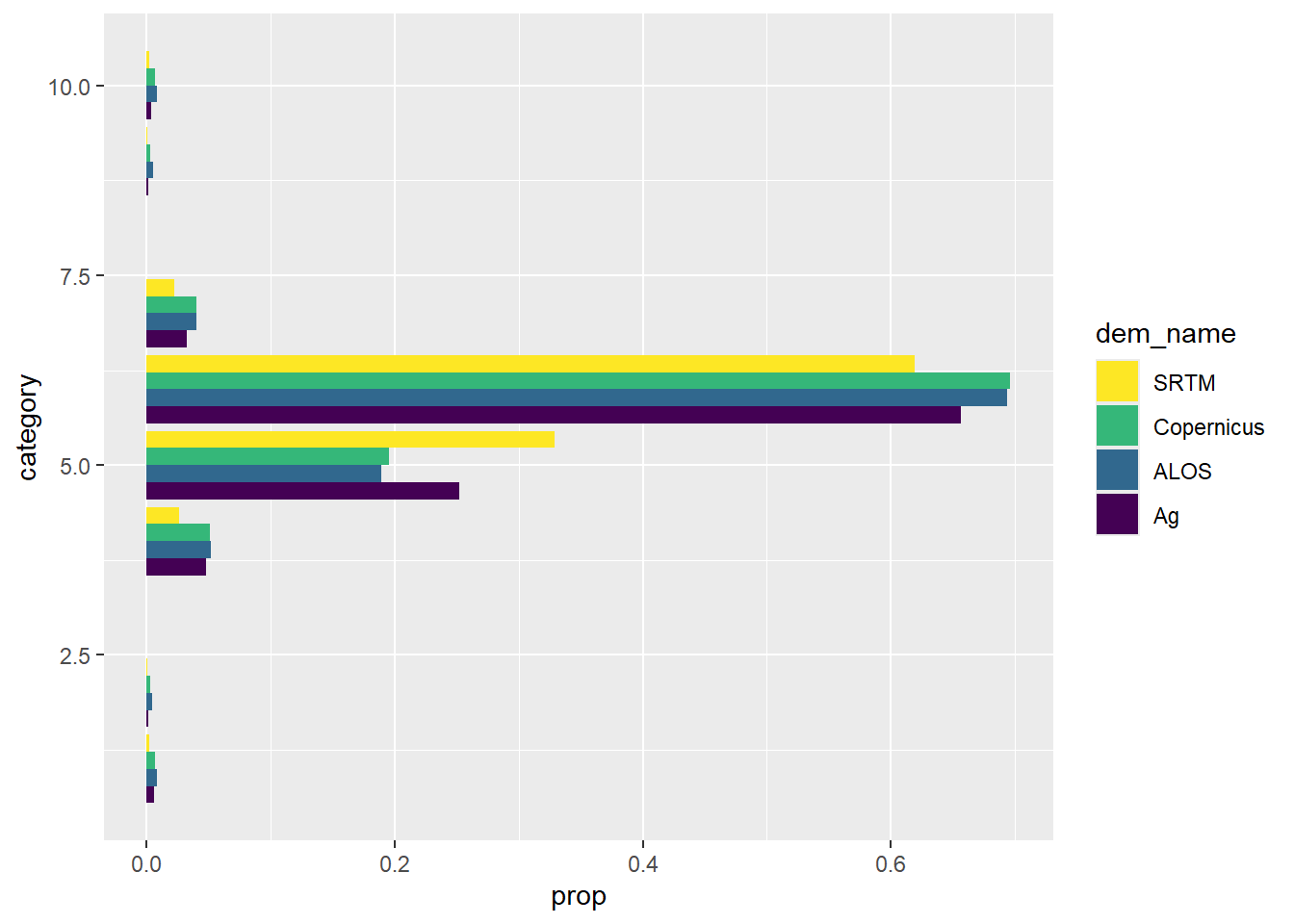
Figure 8.42: Proportion of categorised Deep Creek area in each of several classification classes