5 Cleland
5.1 Continuous
5.1.1 elev
Figure 5.1 shows rasters for elev in the Cleland area.
Table 5.2 shows boxplots for each decile of elev, allowing a comparison of values within each DEM across different ranges of elev. Deciles are based on the values in the reference DEM: Ag.
Figure 5.3 shows the a distribution of values for each sample DEM and window size.
Figure 5.4 shows the distribution of differences between the reference DEM and the other DEMs.
Figure 5.1: elev raster for each DEM
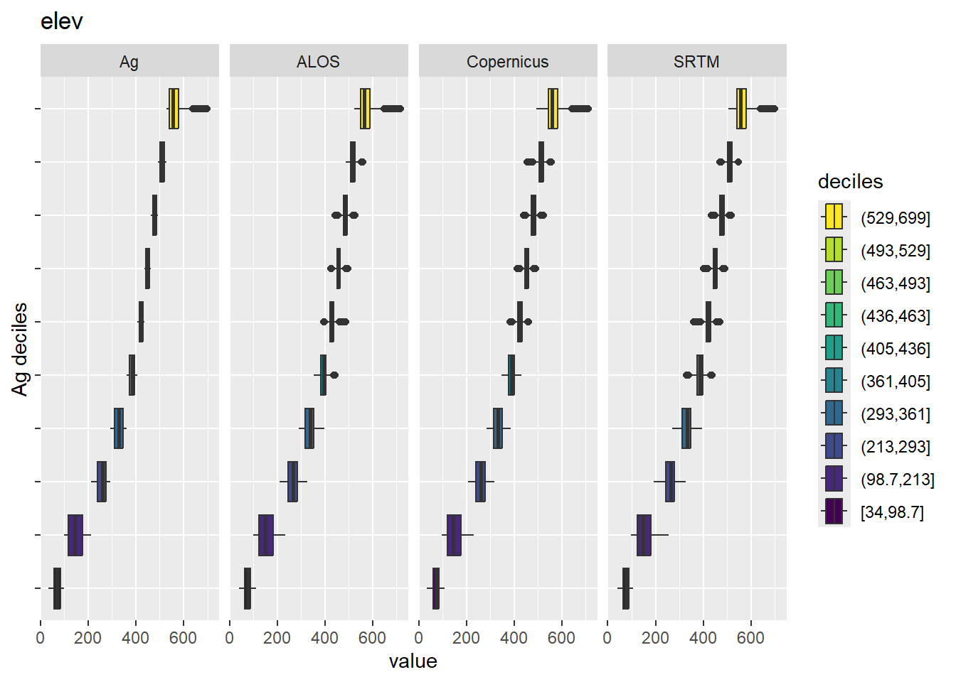
Figure 5.2: Range of values within deciles for each DEM. Deciles are taken from the reference DEM
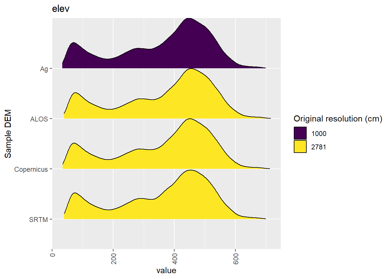
Figure 5.3: Distribution of elev values in each DEM: Cleland
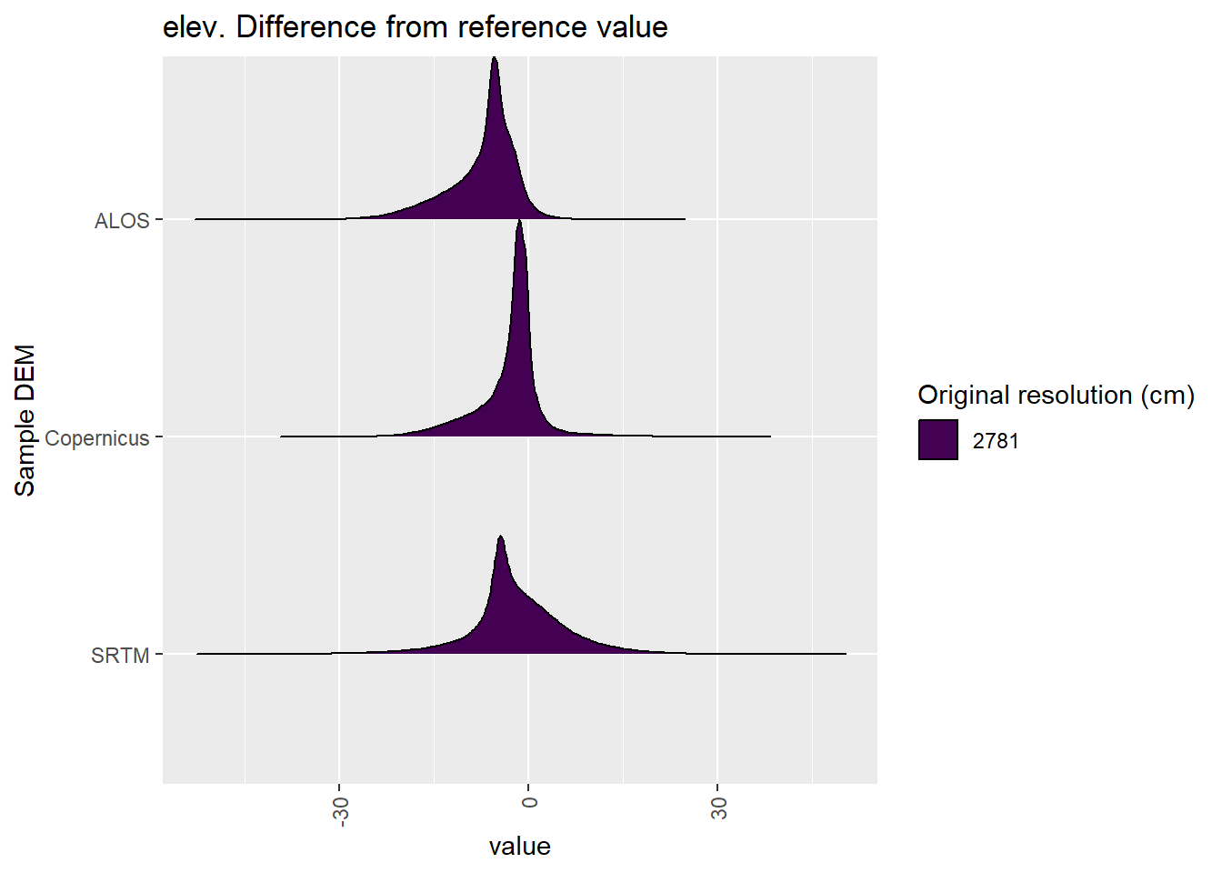
Figure 5.4: Distribution of difference between each DEM and reference for elev values: Cleland
5.1.2 qslope
Figure 5.5 shows rasters for qslope in the Cleland area.
Table 5.6 shows boxplots for each decile of qslope, allowing a comparison of values within each DEM across different ranges of qslope. Deciles are based on the values in the reference DEM: Ag.
Figure 5.7 shows the a distribution of values for each sample DEM and window size.
Figure 5.8 shows the distribution of differences between the reference DEM and the other DEMs.
Figure 5.5: qslope raster for each DEM
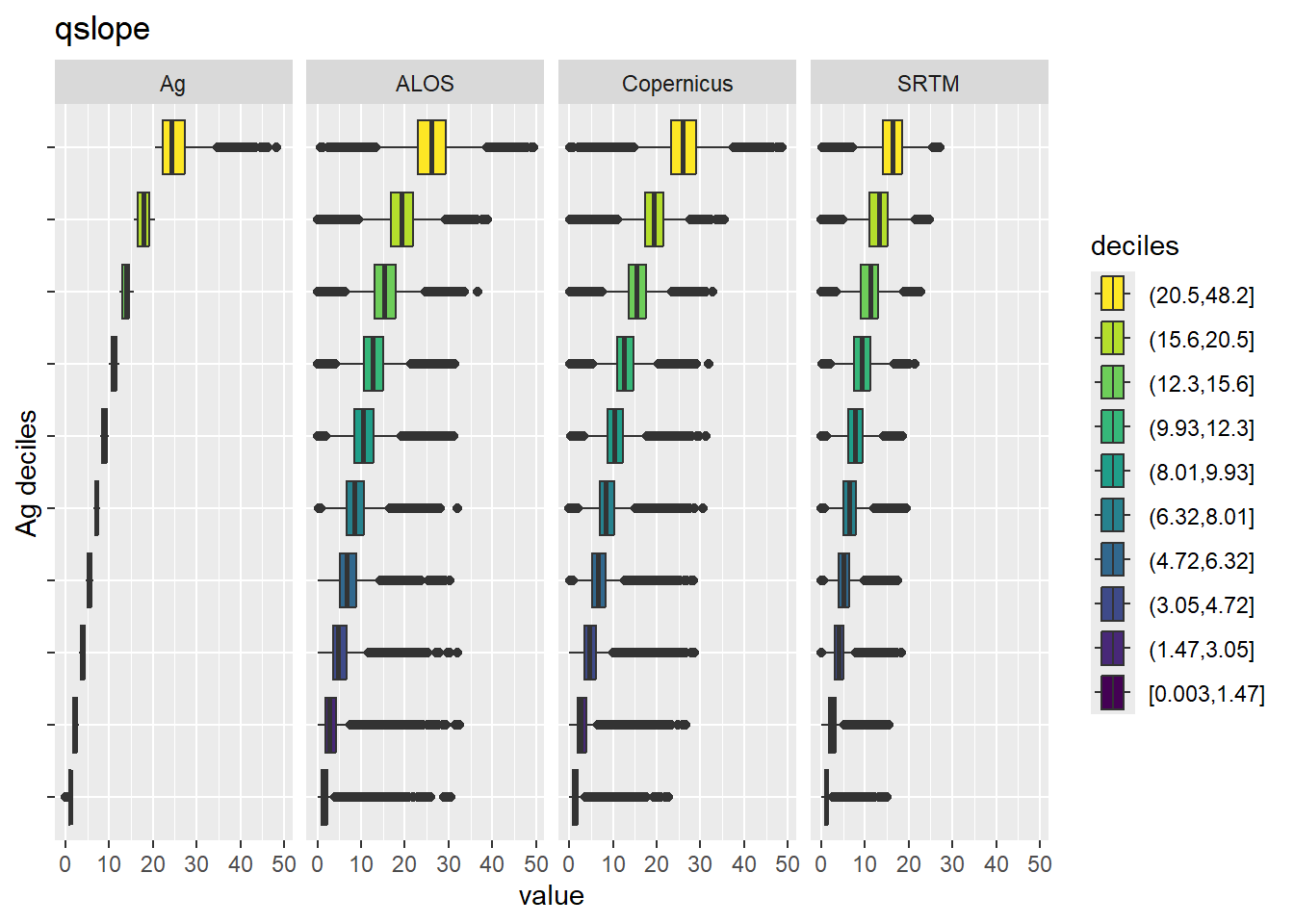
Figure 5.6: Range of values within deciles for each DEM. Deciles are taken from the reference DEM
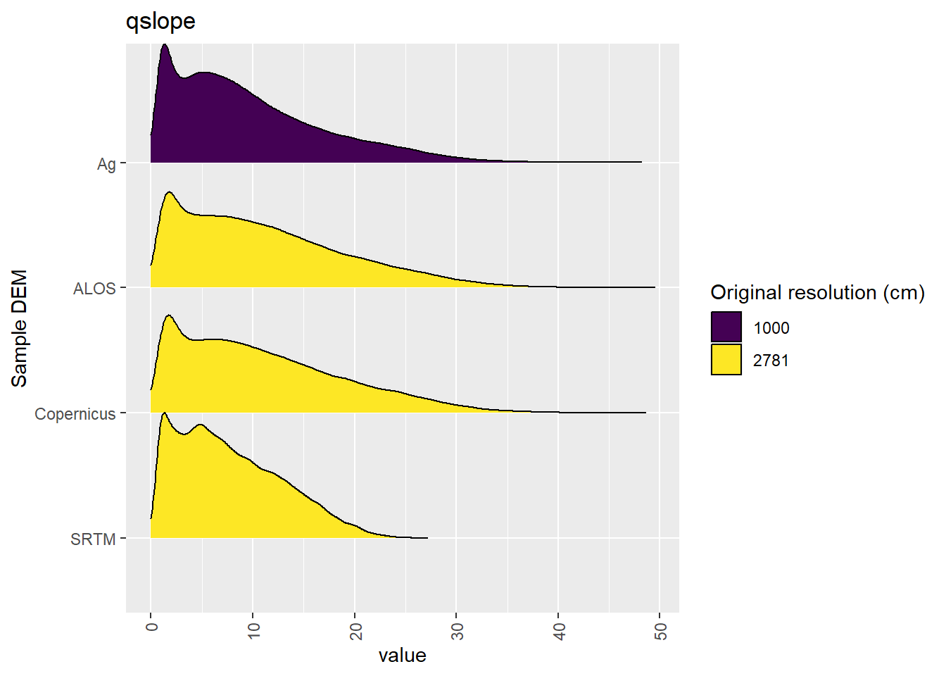
Figure 5.7: Distribution of qslope values in each DEM: Cleland
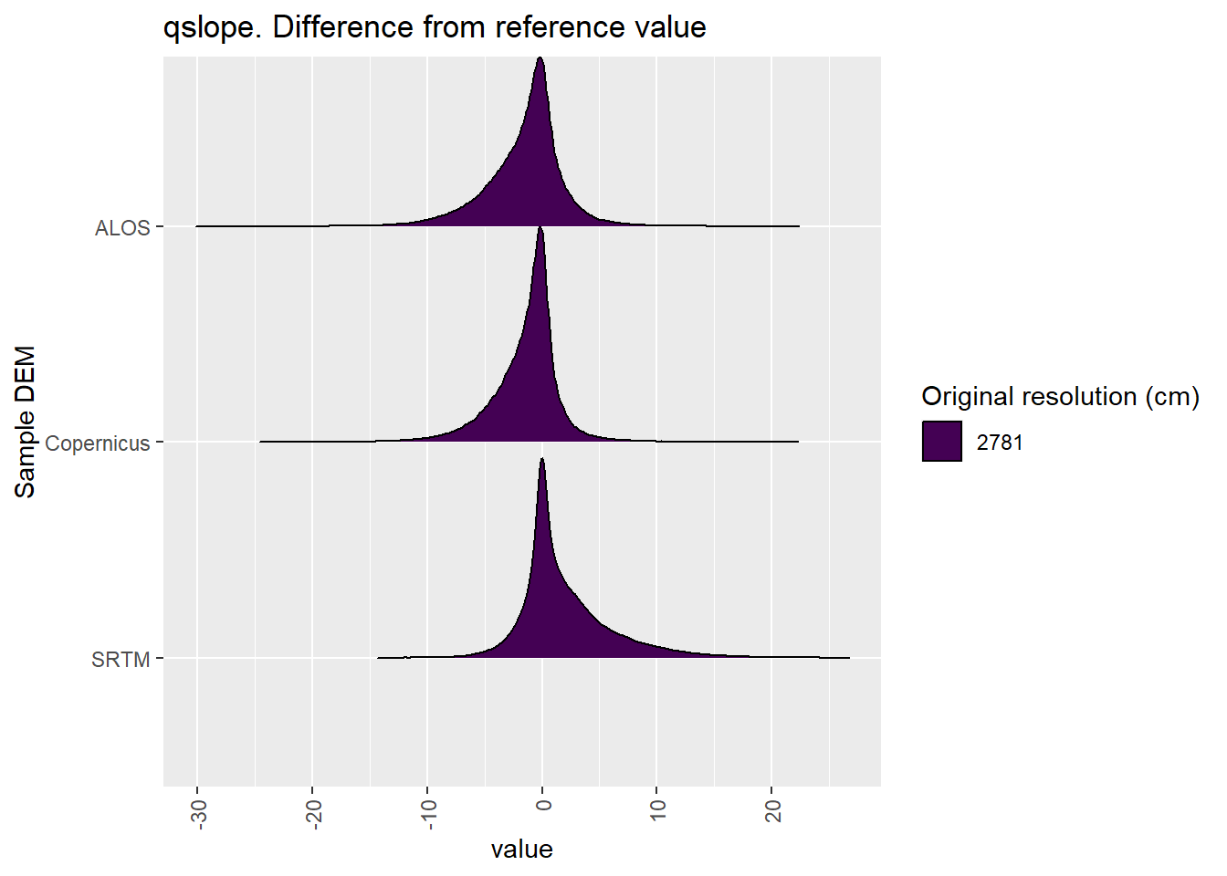
Figure 5.8: Distribution of difference between each DEM and reference for qslope values: Cleland
5.1.3 qaspect
Figure 5.9 shows rasters for qaspect in the Cleland area.
Table 5.10 shows boxplots for each decile of qaspect, allowing a comparison of values within each DEM across different ranges of qaspect. Deciles are based on the values in the reference DEM: Ag.
Figure 5.11 shows the a distribution of values for each sample DEM and window size.
Figure 5.12 shows the distribution of differences between the reference DEM and the other DEMs.
Figure 5.9: qaspect raster for each DEM
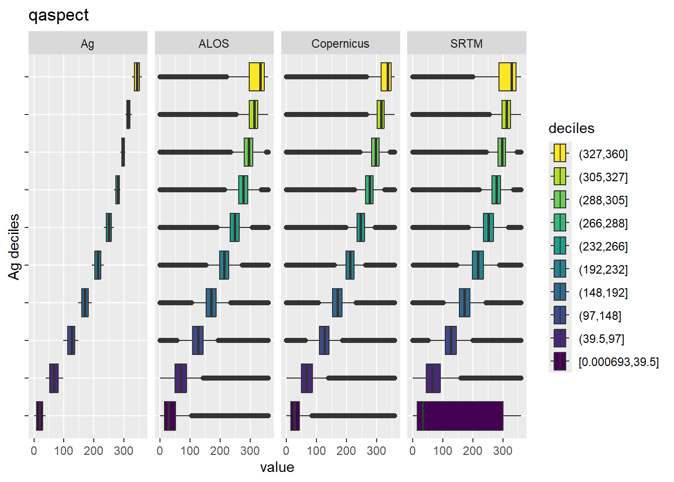
Figure 5.10: Range of values within deciles for each DEM. Deciles are taken from the reference DEM
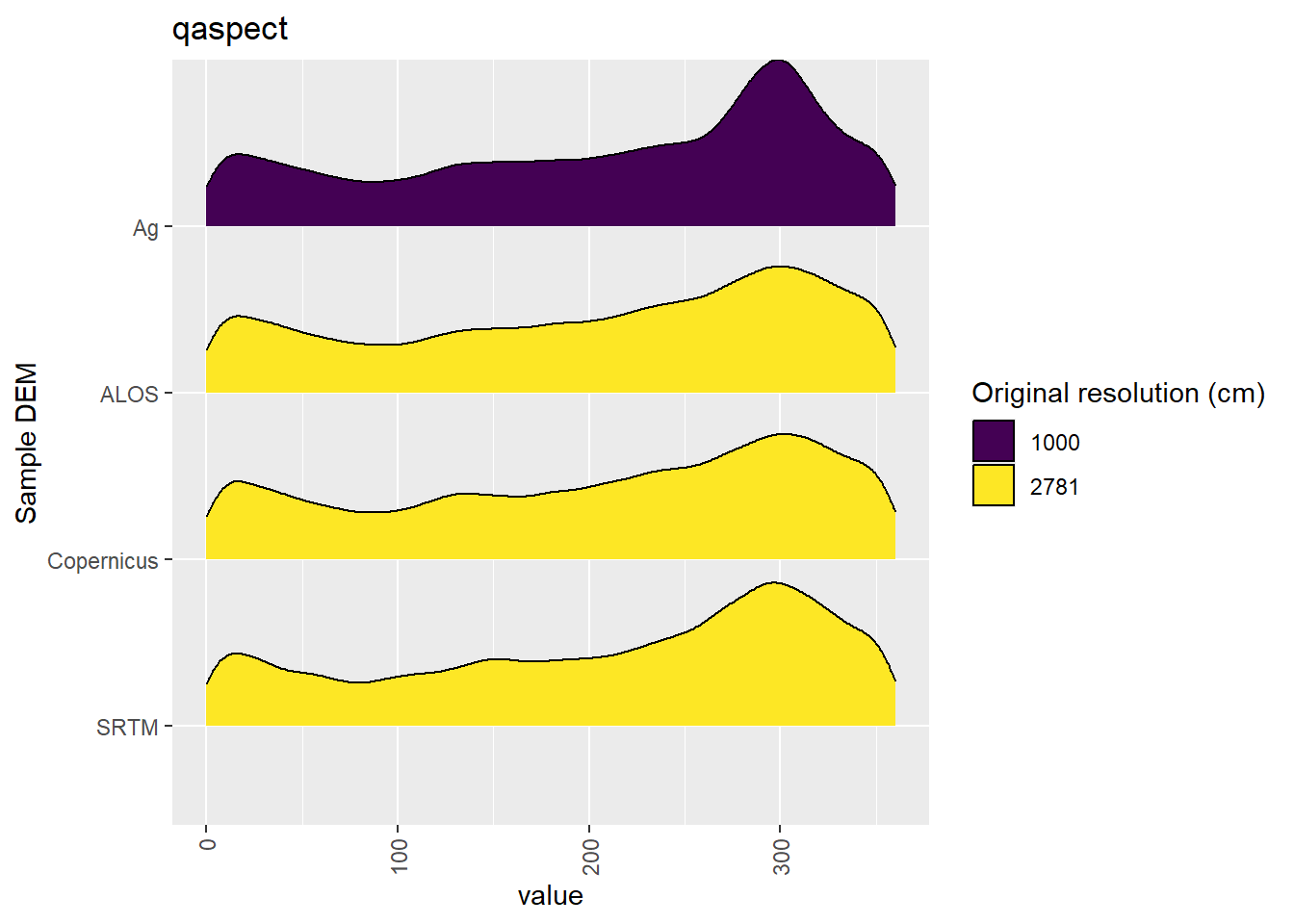
Figure 5.11: Distribution of qaspect values in each DEM: Cleland
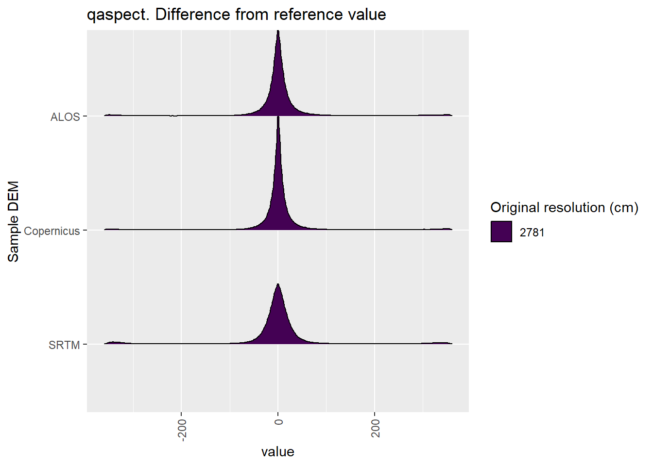
Figure 5.12: Distribution of difference between each DEM and reference for qaspect values: Cleland
5.1.4 qeastness
Figure 5.13 shows rasters for qeastness in the Cleland area.
Table 5.14 shows boxplots for each decile of qeastness, allowing a comparison of values within each DEM across different ranges of qeastness. Deciles are based on the values in the reference DEM: Ag.
Figure 5.15 shows the a distribution of values for each sample DEM and window size.
Figure 5.16 shows the distribution of differences between the reference DEM and the other DEMs.
Figure 5.13: qeastness raster for each DEM
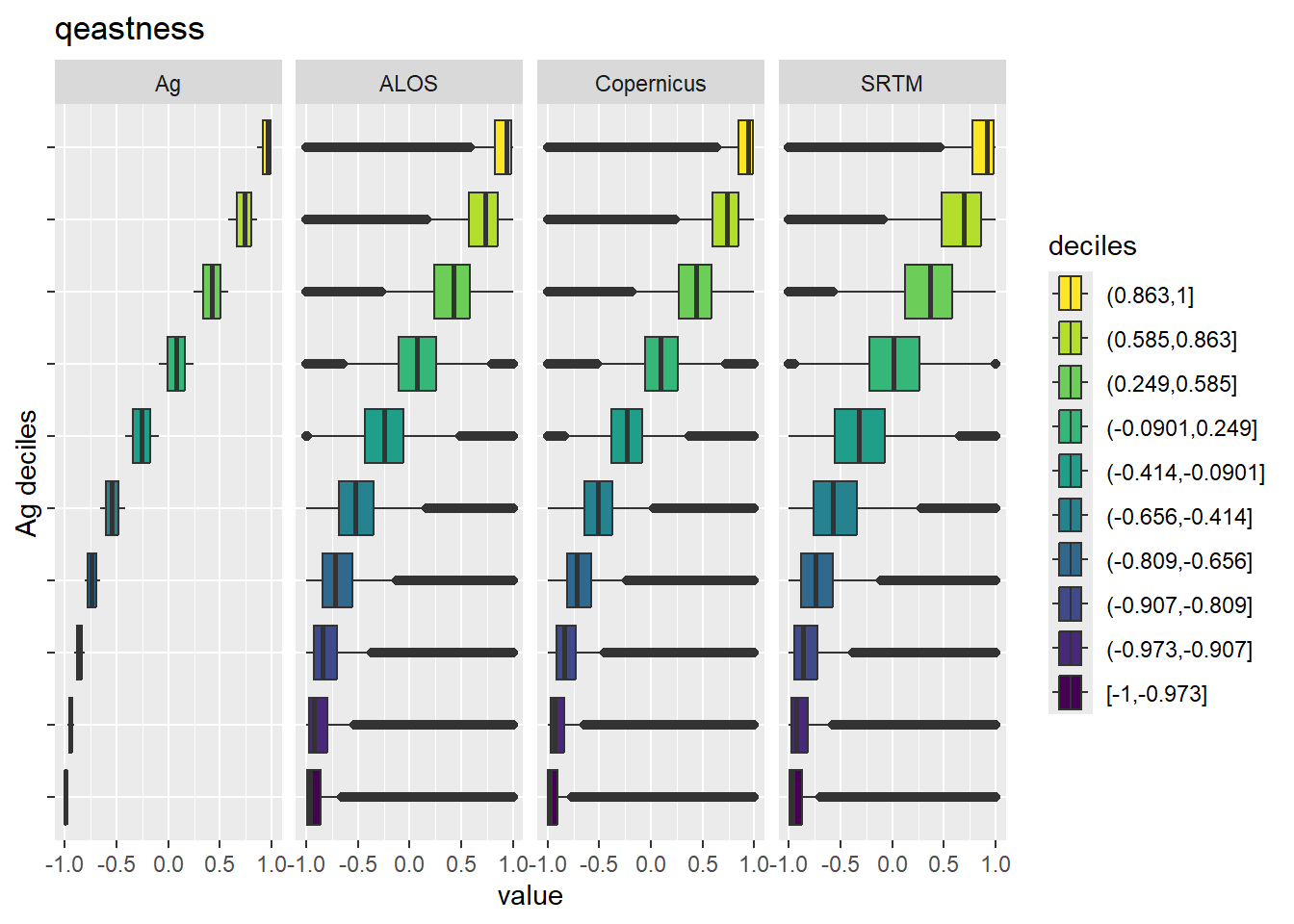
Figure 5.14: Range of values within deciles for each DEM. Deciles are taken from the reference DEM
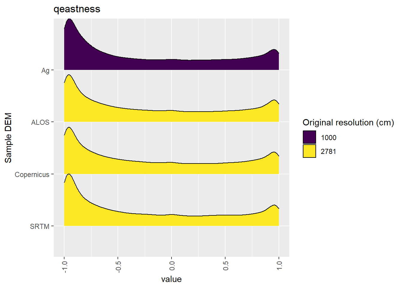
Figure 5.15: Distribution of qeastness values in each DEM: Cleland
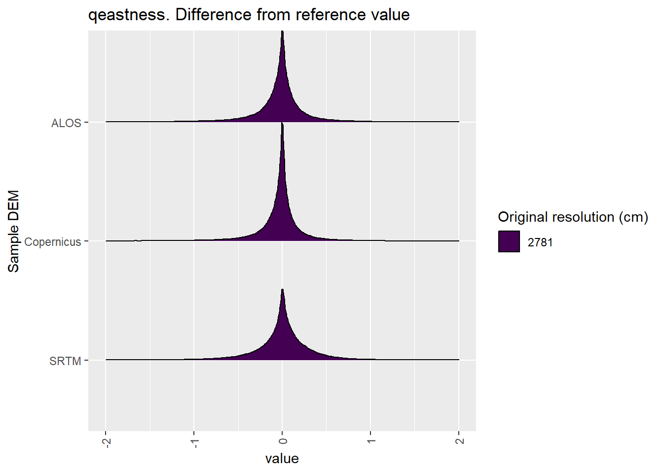
Figure 5.16: Distribution of difference between each DEM and reference for qeastness values: Cleland
5.1.5 qnorthness
Figure 5.17 shows rasters for qnorthness in the Cleland area.
Table 5.18 shows boxplots for each decile of qnorthness, allowing a comparison of values within each DEM across different ranges of qnorthness. Deciles are based on the values in the reference DEM: Ag.
Figure 5.19 shows the a distribution of values for each sample DEM and window size.
Figure 5.20 shows the distribution of differences between the reference DEM and the other DEMs.
Figure 5.17: qnorthness raster for each DEM
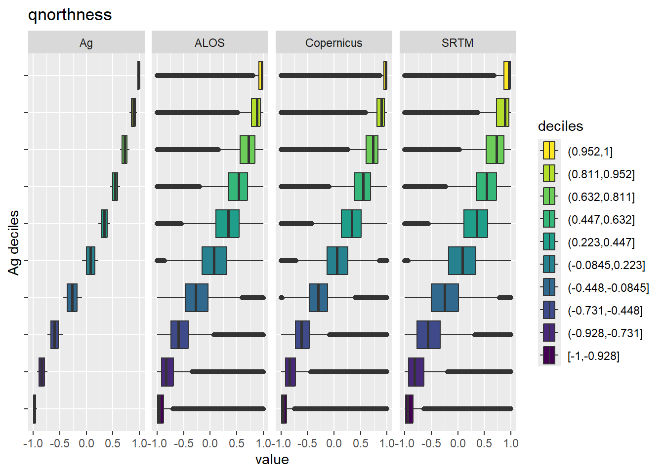
Figure 5.18: Range of values within deciles for each DEM. Deciles are taken from the reference DEM
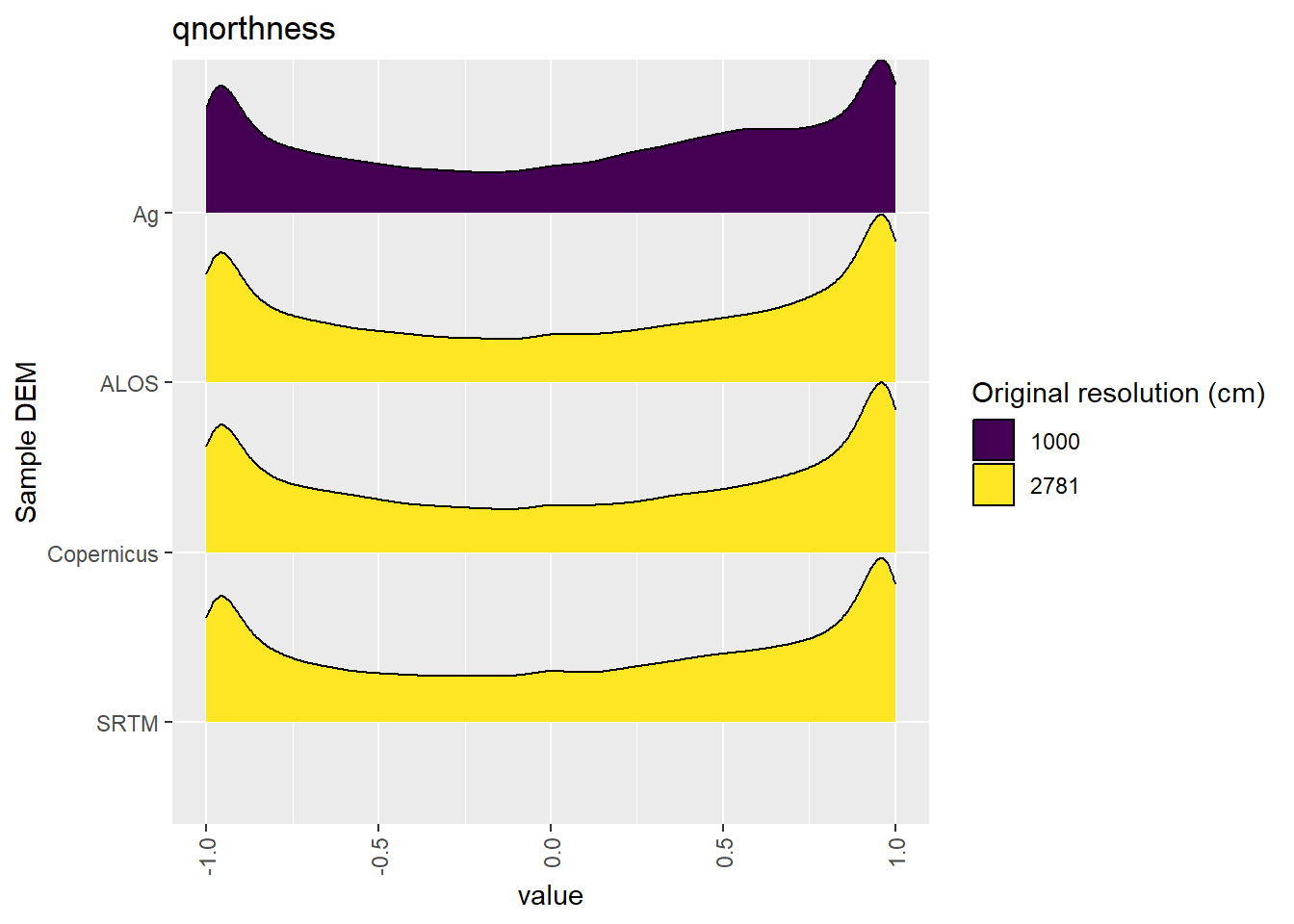
Figure 5.19: Distribution of qnorthness values in each DEM: Cleland
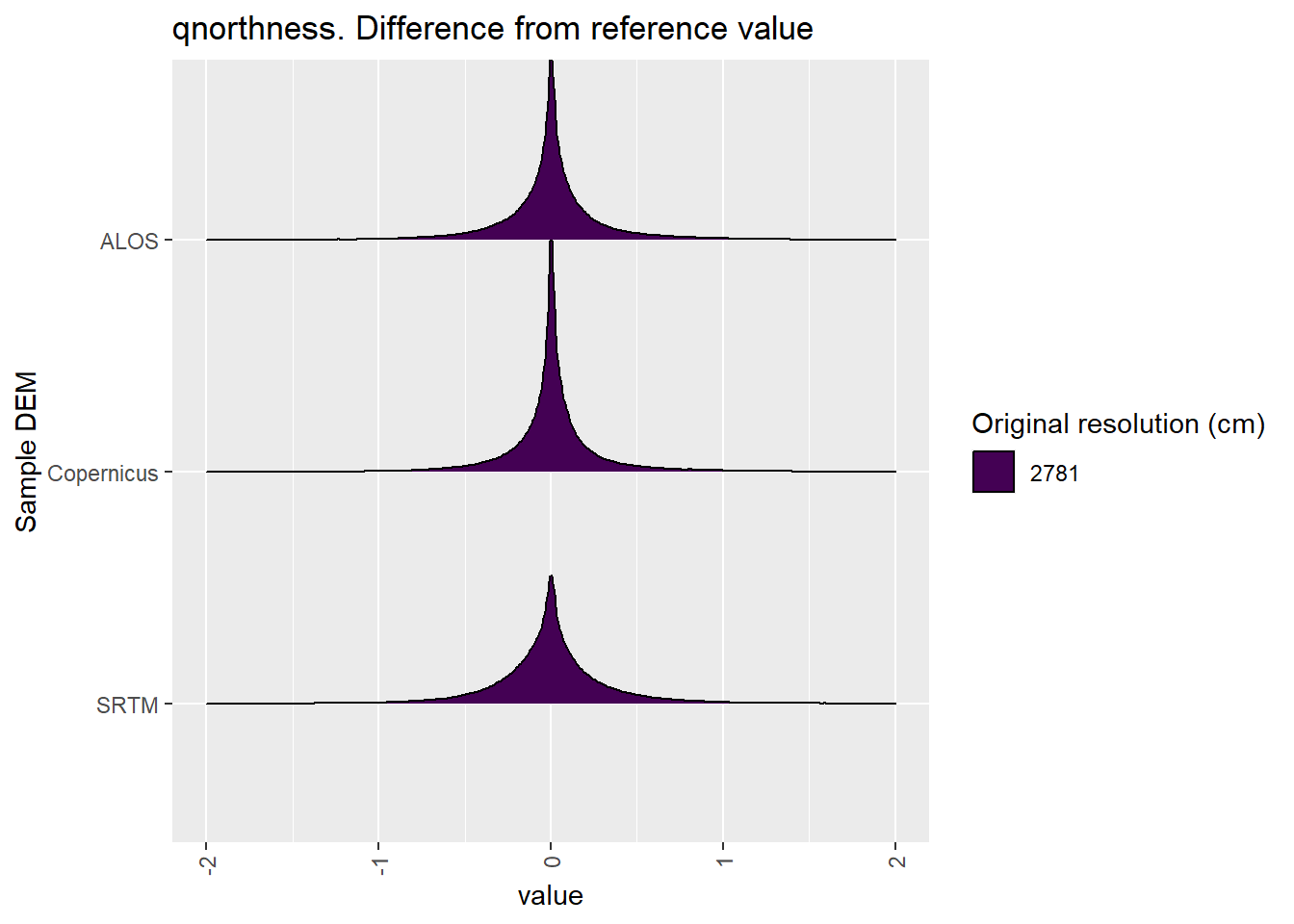
Figure 5.20: Distribution of difference between each DEM and reference for qnorthness values: Cleland
5.1.6 TPI
Figure 5.21 shows rasters for TPI in the Cleland area.
Table 5.22 shows boxplots for each decile of TPI, allowing a comparison of values within each DEM across different ranges of TPI. Deciles are based on the values in the reference DEM: Ag.
Figure 5.23 shows the a distribution of values for each sample DEM and window size.
Figure 5.24 shows the distribution of differences between the reference DEM and the other DEMs.
Figure 5.21: TPI raster for each DEM
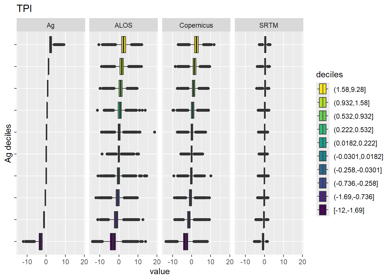
Figure 5.22: Range of values within deciles for each DEM. Deciles are taken from the reference DEM
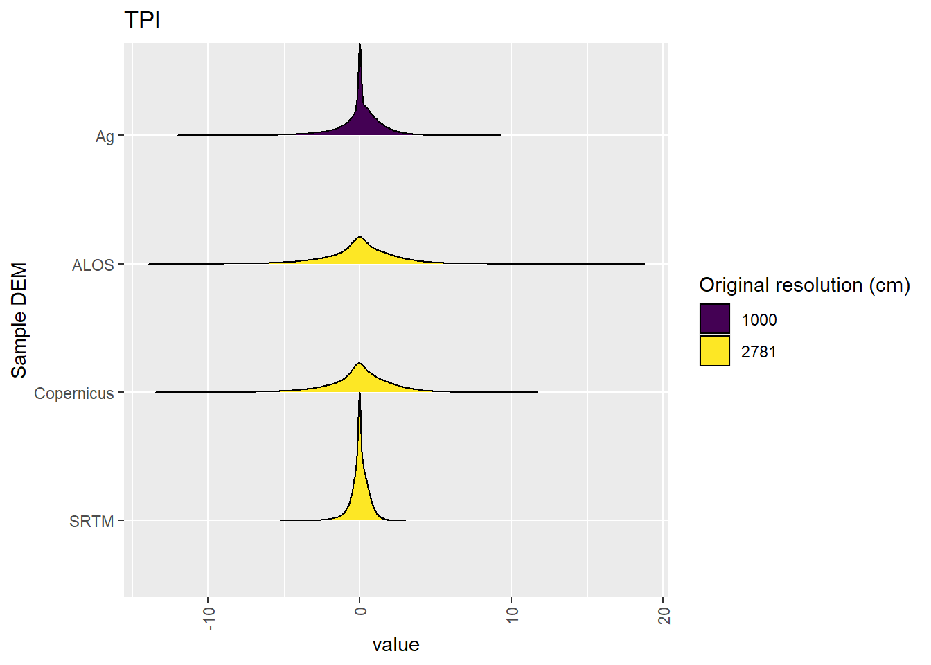
Figure 5.23: Distribution of TPI values in each DEM: Cleland
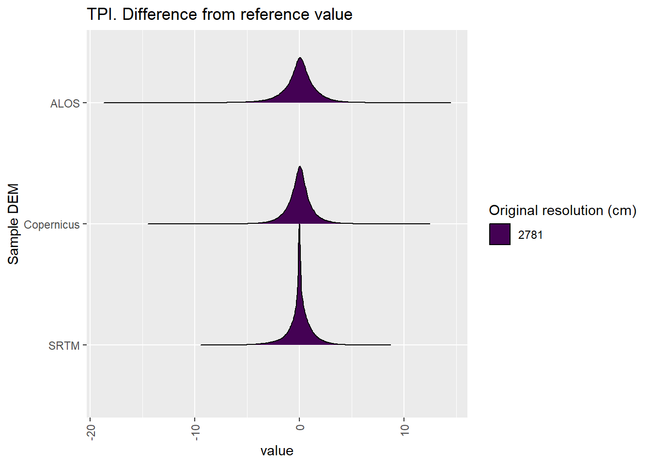
Figure 5.24: Distribution of difference between each DEM and reference for TPI values: Cleland
5.1.7 TRI
Figure 5.25 shows rasters for TRI in the Cleland area.
Table 5.26 shows boxplots for each decile of TRI, allowing a comparison of values within each DEM across different ranges of TRI. Deciles are based on the values in the reference DEM: Ag.
Figure 5.27 shows the a distribution of values for each sample DEM and window size.
Figure 5.28 shows the distribution of differences between the reference DEM and the other DEMs.
Figure 5.25: TRI raster for each DEM
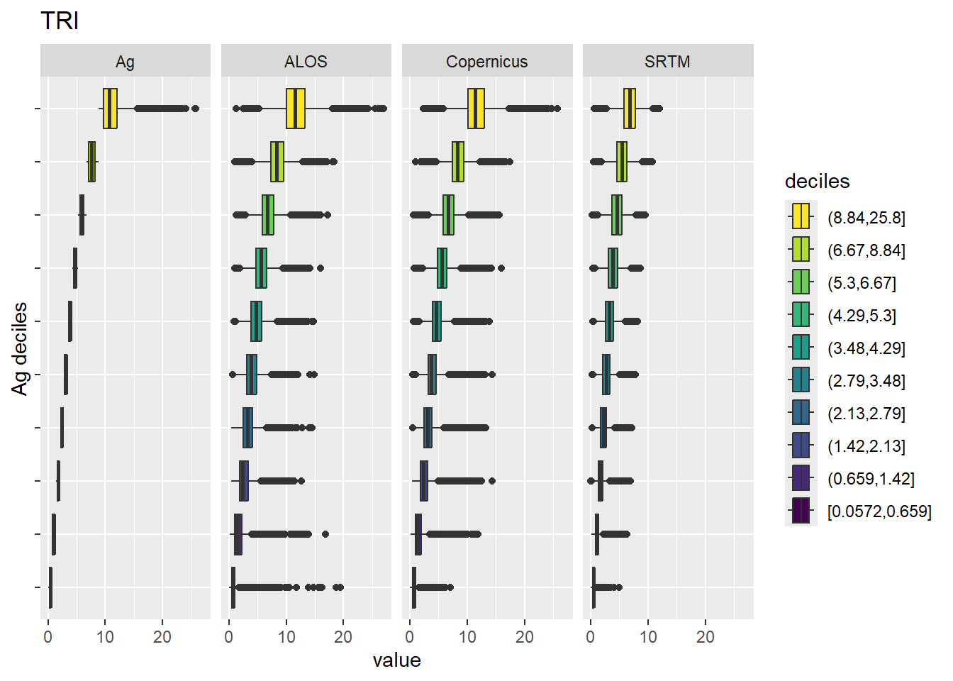
Figure 5.26: Range of values within deciles for each DEM. Deciles are taken from the reference DEM
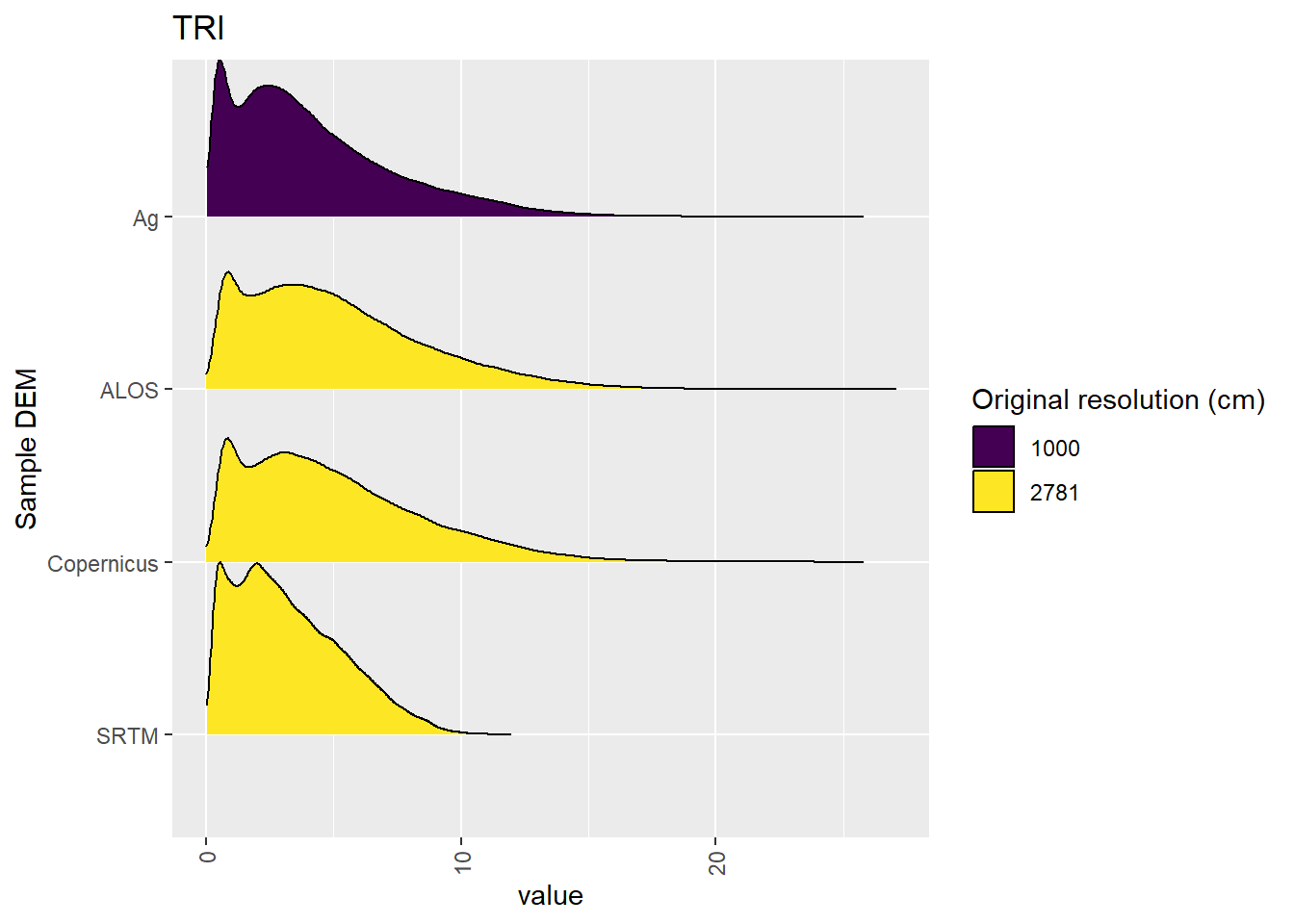
Figure 5.27: Distribution of TRI values in each DEM: Cleland
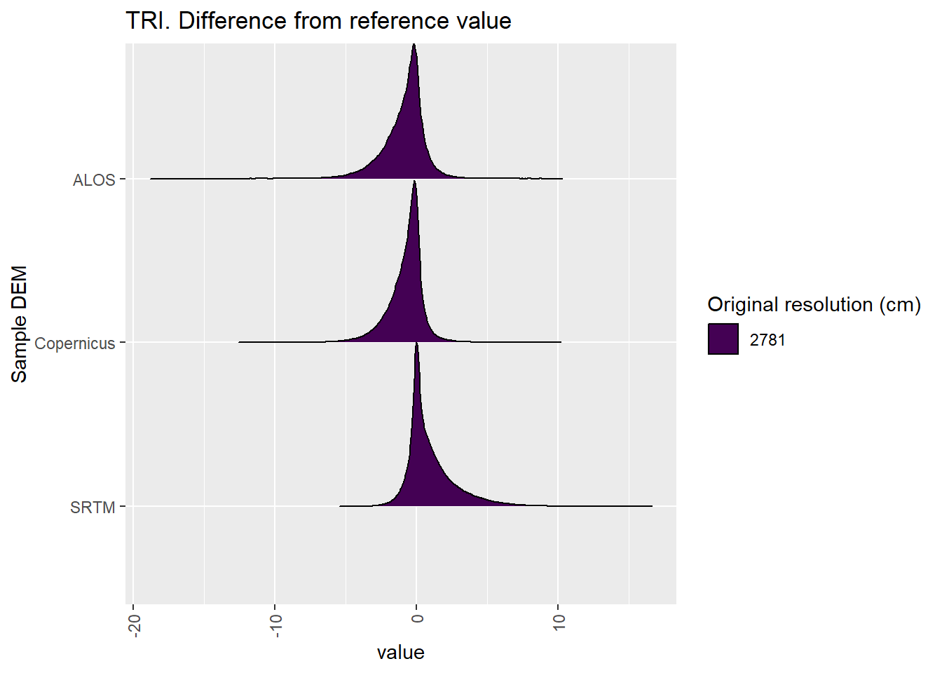
Figure 5.28: Distribution of difference between each DEM and reference for TRI values: Cleland
5.1.8 TRIriley
Figure 5.29 shows rasters for TRIriley in the Cleland area.
Table 5.30 shows boxplots for each decile of TRIriley, allowing a comparison of values within each DEM across different ranges of TRIriley. Deciles are based on the values in the reference DEM: Ag.
Figure 5.31 shows the a distribution of values for each sample DEM and window size.
Figure 5.32 shows the distribution of differences between the reference DEM and the other DEMs.
Figure 5.29: TRIriley raster for each DEM
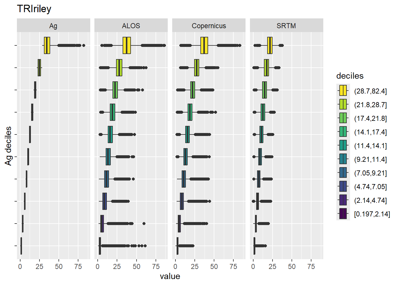
Figure 5.30: Range of values within deciles for each DEM. Deciles are taken from the reference DEM

Figure 5.31: Distribution of TRIriley values in each DEM: Cleland

Figure 5.32: Distribution of difference between each DEM and reference for TRIriley values: Cleland
5.1.9 TRIrmsd
Figure 5.33 shows rasters for TRIrmsd in the Cleland area.
Table 5.34 shows boxplots for each decile of TRIrmsd, allowing a comparison of values within each DEM across different ranges of TRIrmsd. Deciles are based on the values in the reference DEM: Ag.
Figure 5.35 shows the a distribution of values for each sample DEM and window size.
Figure 5.36 shows the distribution of differences between the reference DEM and the other DEMs.
Figure 5.33: TRIrmsd raster for each DEM
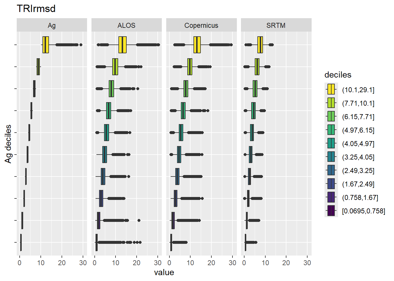
Figure 5.34: Range of values within deciles for each DEM. Deciles are taken from the reference DEM
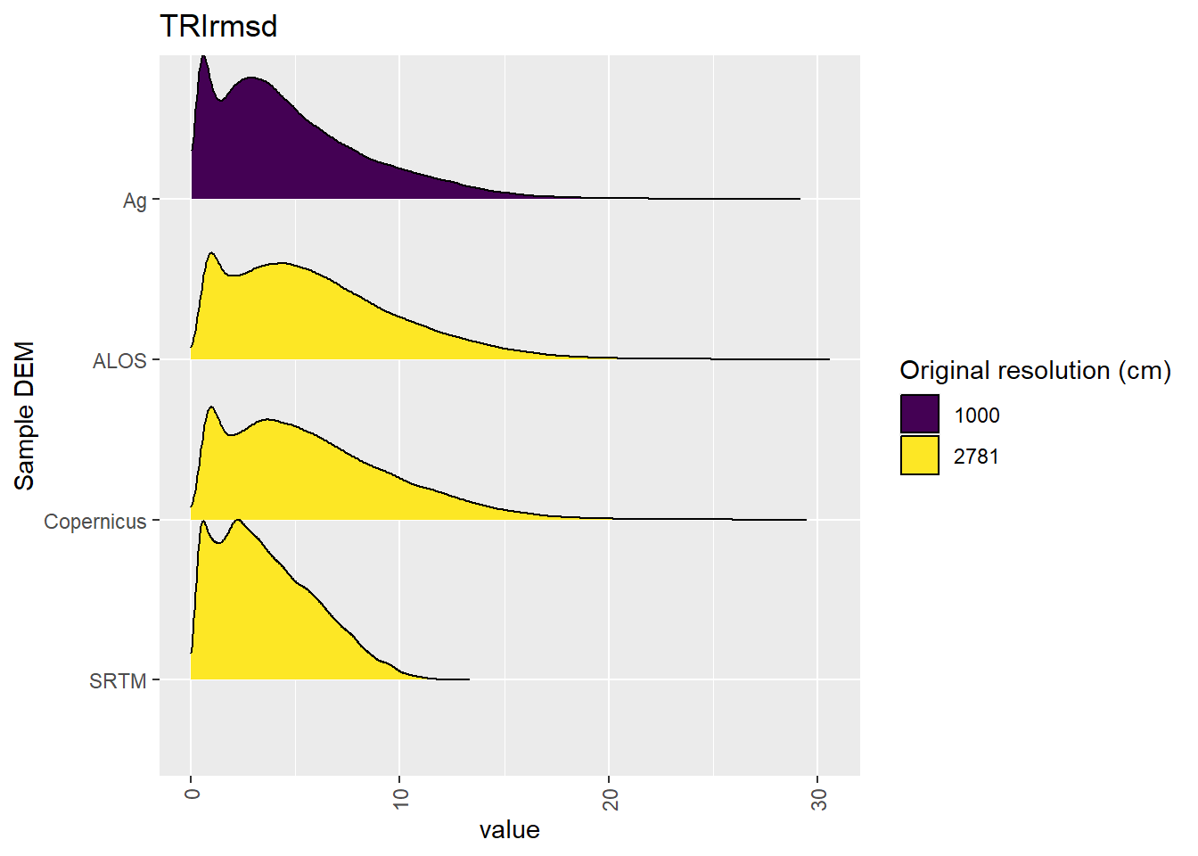
Figure 5.35: Distribution of TRIrmsd values in each DEM: Cleland

Figure 5.36: Distribution of difference between each DEM and reference for TRIrmsd values: Cleland
5.1.10 roughness
Figure 5.37 shows rasters for roughness in the Cleland area.
Table 5.38 shows boxplots for each decile of roughness, allowing a comparison of values within each DEM across different ranges of roughness. Deciles are based on the values in the reference DEM: Ag.
Figure 5.39 shows the a distribution of values for each sample DEM and window size.
Figure 5.40 shows the distribution of differences between the reference DEM and the other DEMs.
Figure 5.37: roughness raster for each DEM
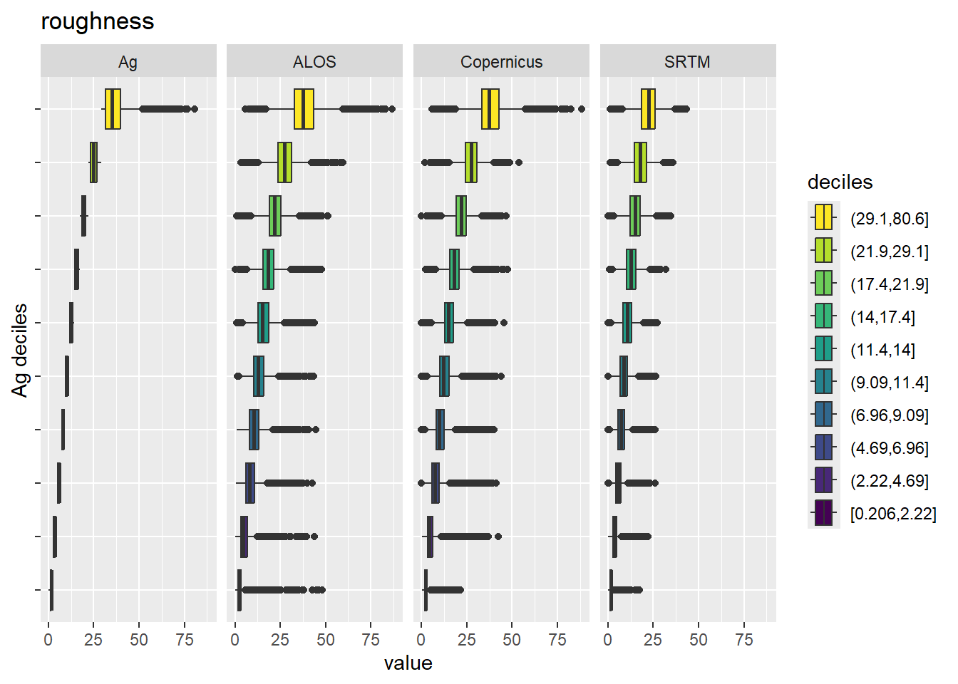
Figure 5.38: Range of values within deciles for each DEM. Deciles are taken from the reference DEM
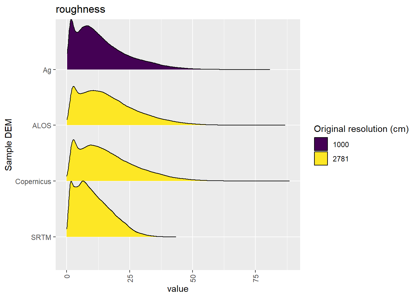
Figure 5.39: Distribution of roughness values in each DEM: Cleland
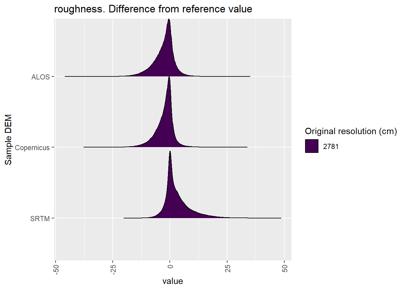
Figure 5.40: Distribution of difference between each DEM and reference for roughness values: Cleland
5.2 Categorical
Table 5.1 shows the proportion of each DEM classifed to each landform element (also see Figure 5.42.
Figure 5.41 shows a landscape classification for each reprojected area.
| landform | Ag | ALOS | Copernicus | SRTM |
|---|---|---|---|---|
| canyon | 0.0054 | 0.0083157 | 0.007680 | 0.00124 |
| midslope drainage | 0.0016 | 0.0092072 | 0.007529 | 0.00019 |
| upland drainage | 0.0000091 | 0.000018 | ||
| u-shaped valley | 0.0386 | 0.0486598 | 0.045670 | 0.01656 |
| plains | 0.2772 | 0.2117279 | 0.214539 | 0.32417 |
| open slopes | 0.6458 | 0.6646201 | 0.669324 | 0.63670 |
| upper slopes | 0.0270 | 0.0382778 | 0.039348 | 0.01921 |
| midslopes ridges | 0.0014 | 0.0101672 | 0.008526 | 0.00022 |
| mountain tops | 0.0030 | 0.0090151 | 0.007365 | 0.00170 |
Figure 5.41: Categorical representation of Cleland
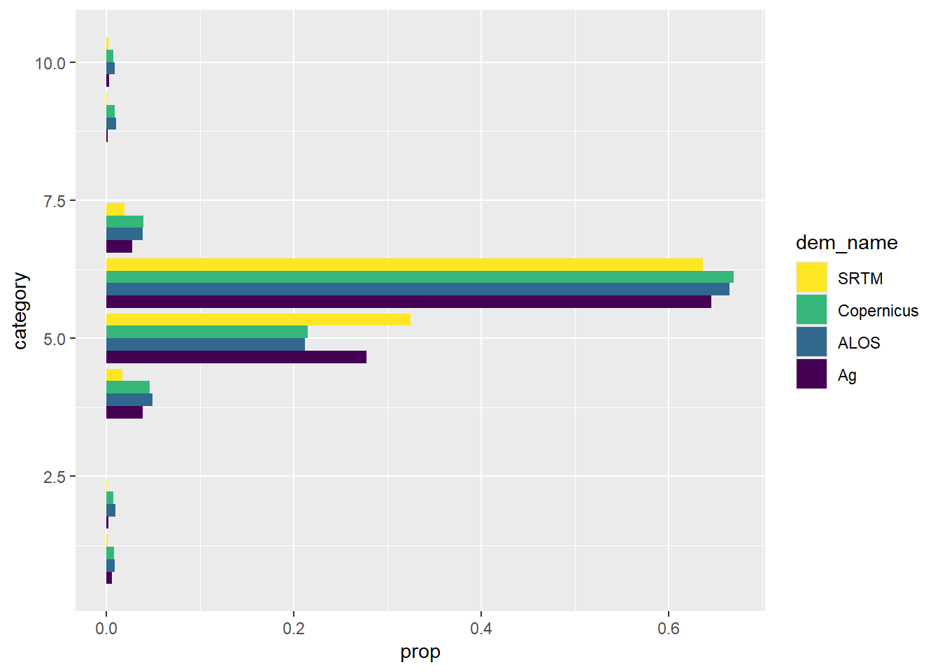
Figure 5.42: Proportion of categorised Cleland area in each of several classification classes