9 Algebuckina
9.1 Continuous
9.1.1 elev
Figure 9.1 shows rasters for elev in the Algebuckina area.
Table 9.2 shows boxplots for each decile of elev, allowing a comparison of values within each DEM across different ranges of elev. Deciles are based on the values in the reference DEM: Outback.
Figure 9.3 shows the a distribution of values for each sample DEM and window size.
Figure 9.4 shows the distribution of differences between the reference DEM and the other DEMs.
Figure 9.1: elev raster for each DEM
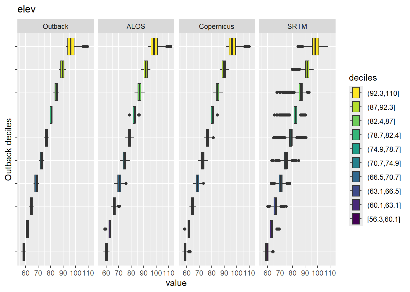
Figure 9.2: Range of values within deciles for each DEM. Deciles are taken from the reference DEM
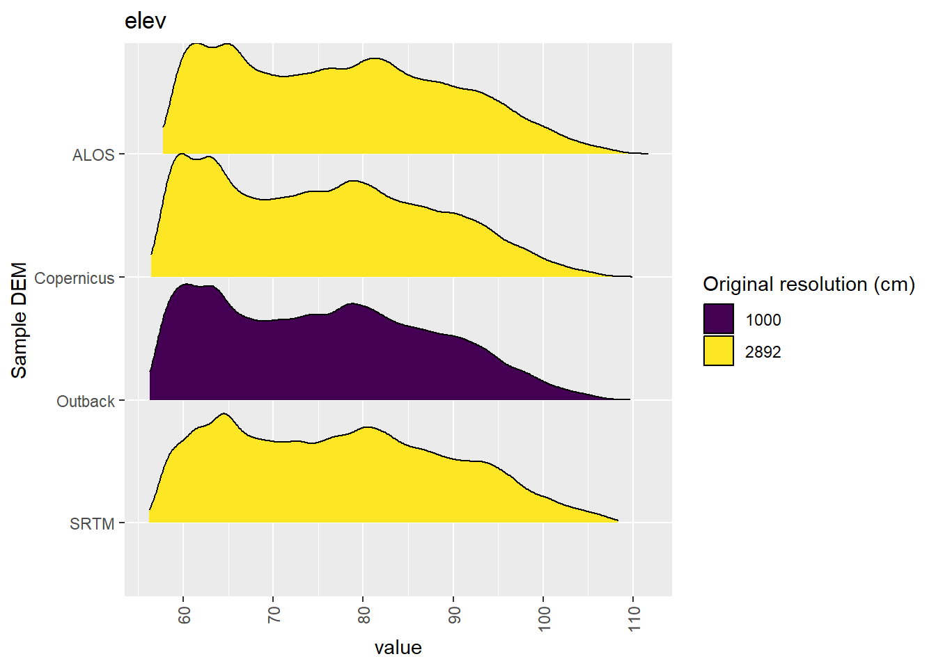
Figure 9.3: Distribution of elev values in each DEM: Algebuckina
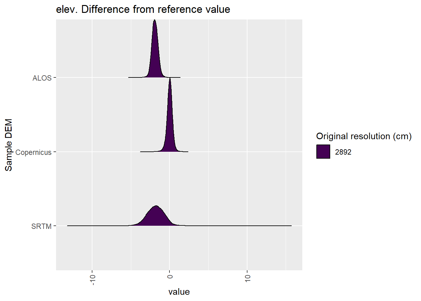
Figure 9.4: Distribution of difference between each DEM and reference for elev values: Algebuckina
9.1.2 qslope
Figure 9.5 shows rasters for qslope in the Algebuckina area.
Table 9.6 shows boxplots for each decile of qslope, allowing a comparison of values within each DEM across different ranges of qslope. Deciles are based on the values in the reference DEM: Outback.
Figure 9.7 shows the a distribution of values for each sample DEM and window size.
Figure 9.8 shows the distribution of differences between the reference DEM and the other DEMs.
Figure 9.5: qslope raster for each DEM
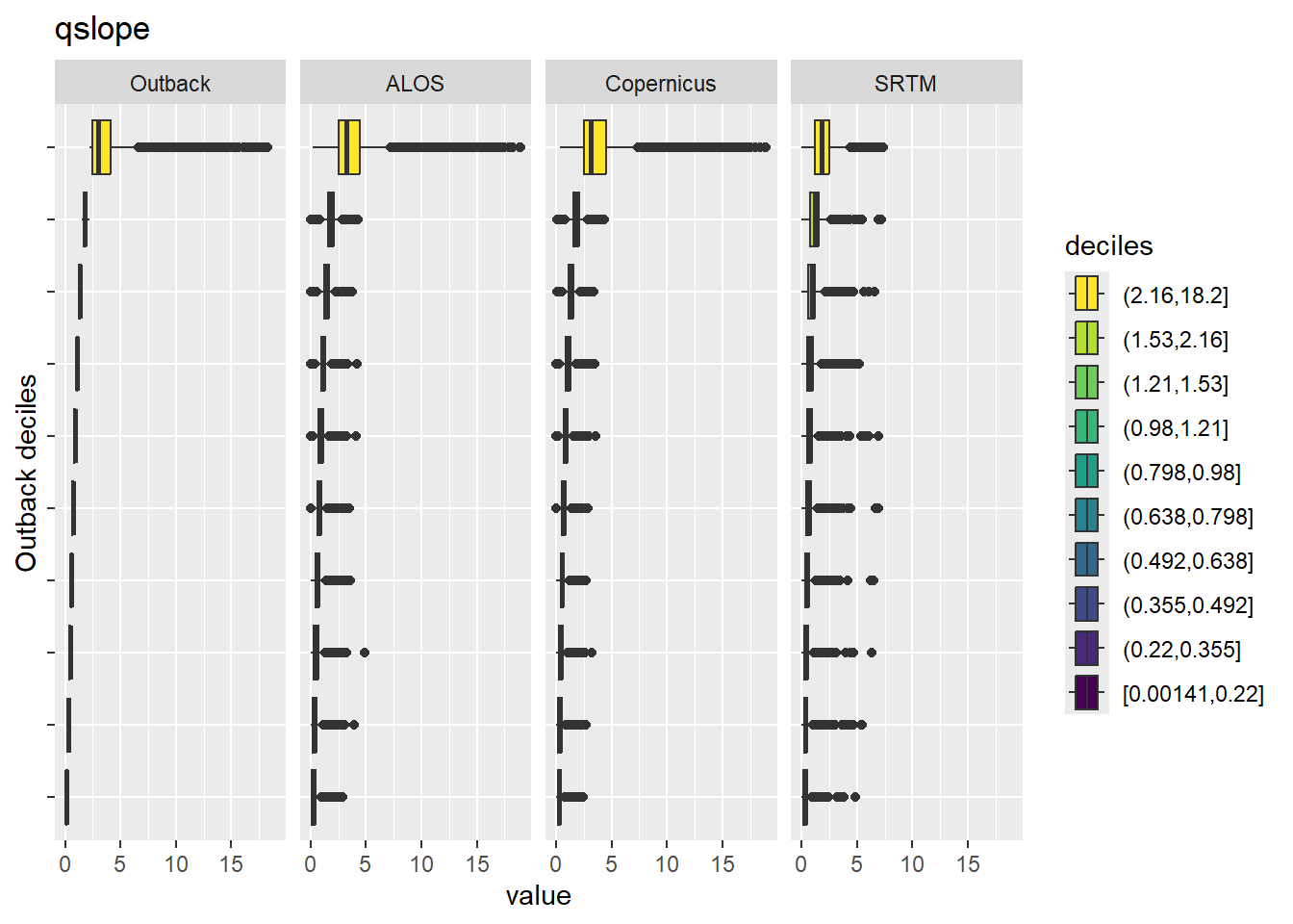
Figure 9.6: Range of values within deciles for each DEM. Deciles are taken from the reference DEM
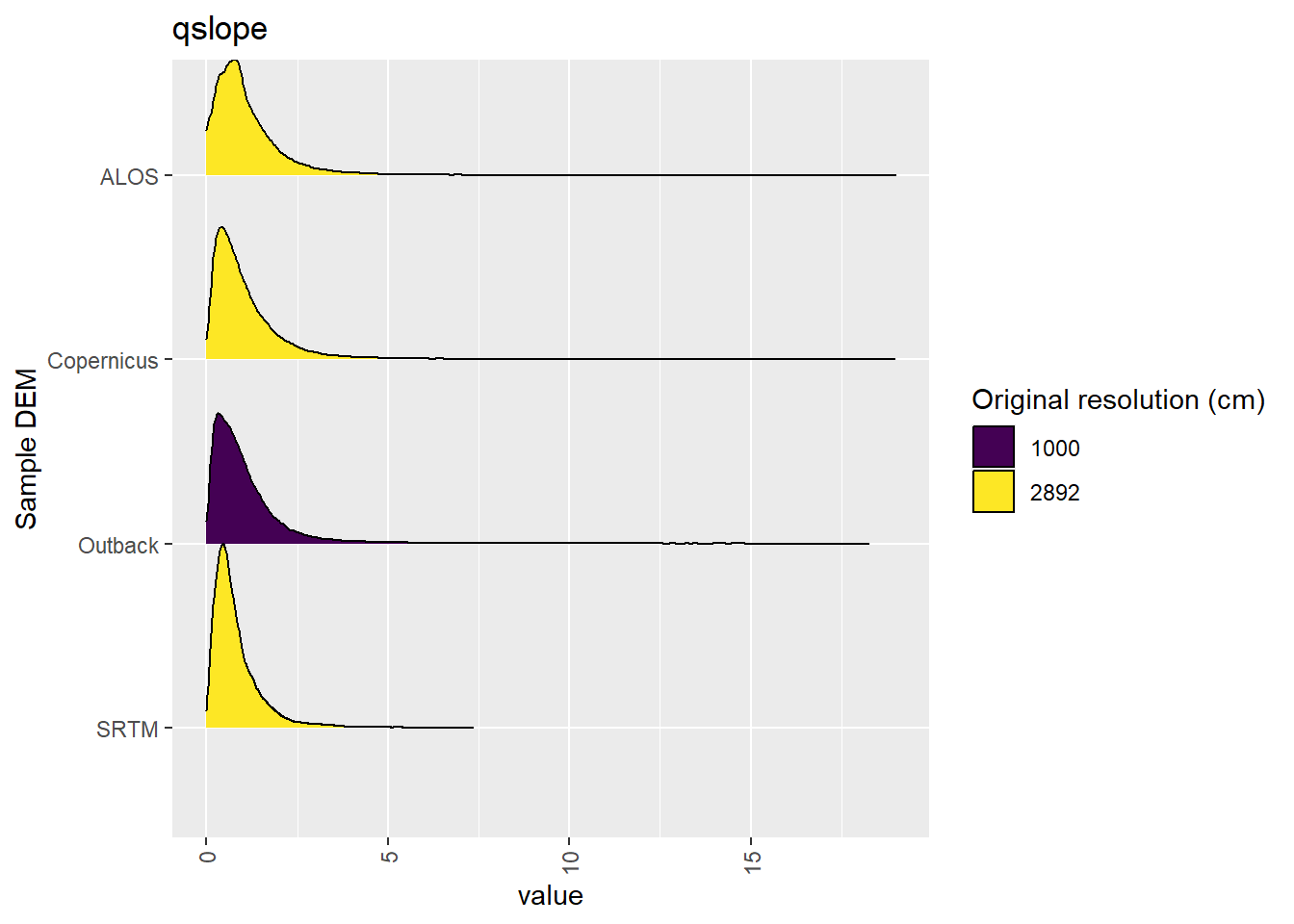
Figure 9.7: Distribution of qslope values in each DEM: Algebuckina
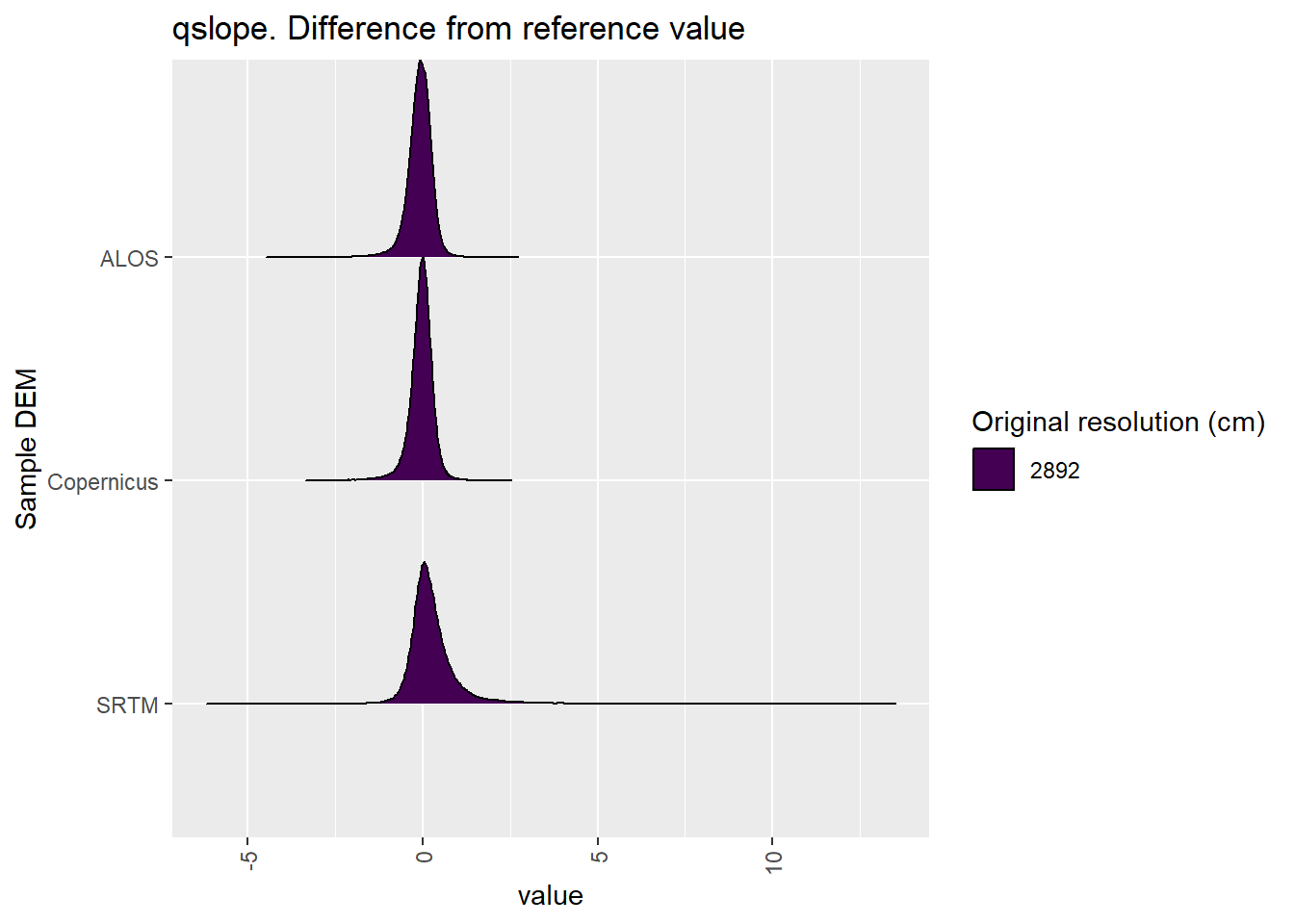
Figure 9.8: Distribution of difference between each DEM and reference for qslope values: Algebuckina
9.1.3 qaspect
Figure 9.9 shows rasters for qaspect in the Algebuckina area.
Table 9.10 shows boxplots for each decile of qaspect, allowing a comparison of values within each DEM across different ranges of qaspect. Deciles are based on the values in the reference DEM: Outback.
Figure 9.11 shows the a distribution of values for each sample DEM and window size.
Figure 9.12 shows the distribution of differences between the reference DEM and the other DEMs.
Figure 9.9: qaspect raster for each DEM
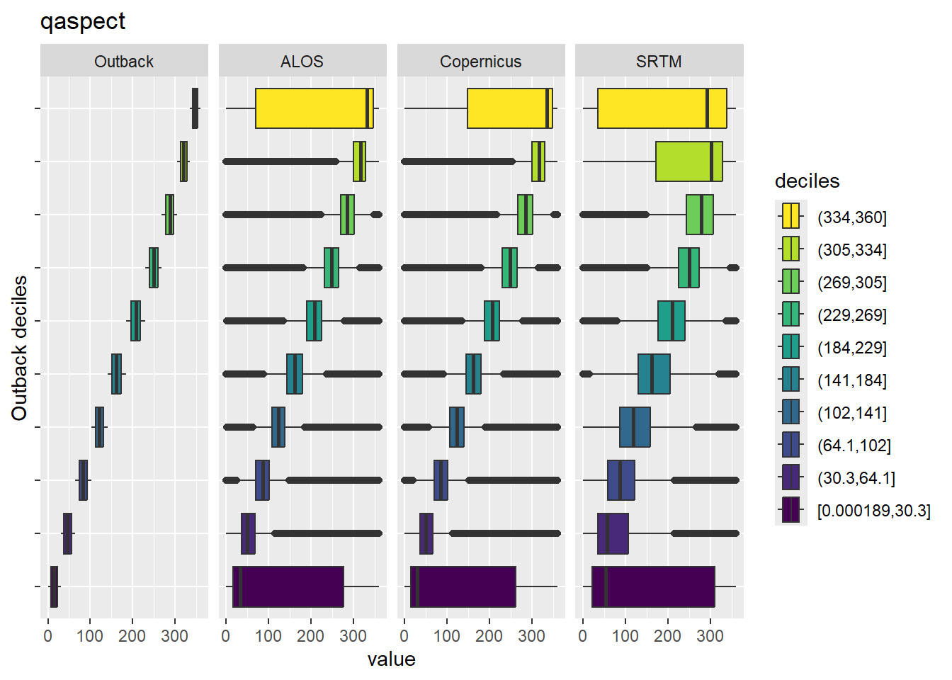
Figure 9.10: Range of values within deciles for each DEM. Deciles are taken from the reference DEM
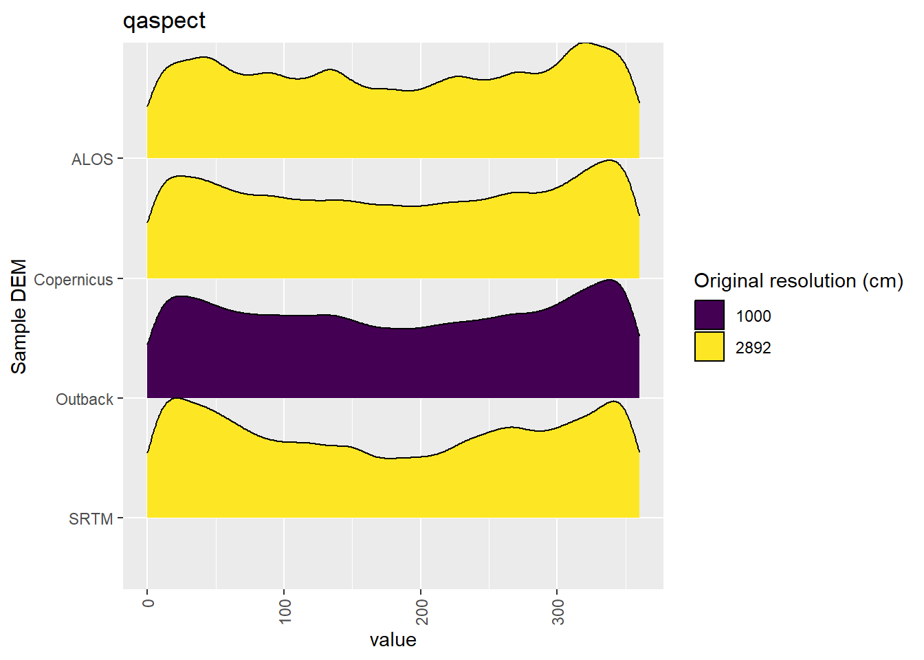
Figure 9.11: Distribution of qaspect values in each DEM: Algebuckina
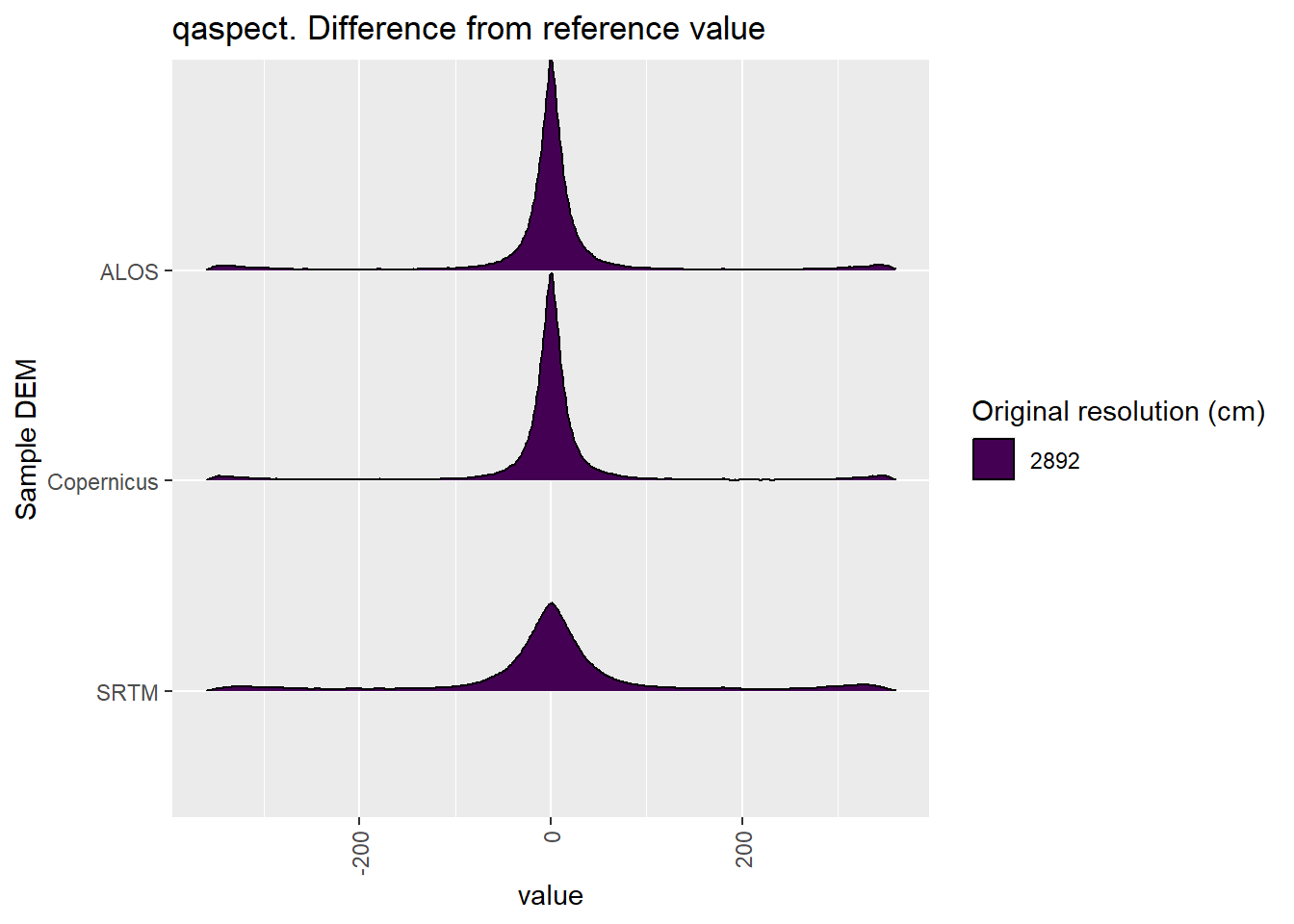
Figure 9.12: Distribution of difference between each DEM and reference for qaspect values: Algebuckina
9.1.4 qeastness
Figure 9.13 shows rasters for qeastness in the Algebuckina area.
Table 9.14 shows boxplots for each decile of qeastness, allowing a comparison of values within each DEM across different ranges of qeastness. Deciles are based on the values in the reference DEM: Outback.
Figure 9.15 shows the a distribution of values for each sample DEM and window size.
Figure 9.16 shows the distribution of differences between the reference DEM and the other DEMs.
Figure 9.13: qeastness raster for each DEM
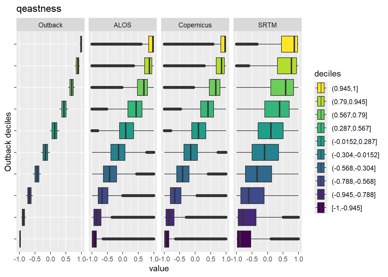
Figure 9.14: Range of values within deciles for each DEM. Deciles are taken from the reference DEM
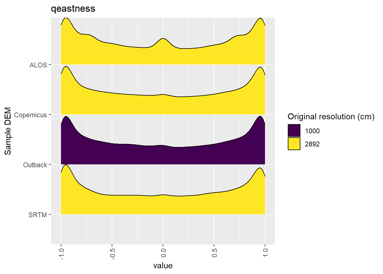
Figure 9.15: Distribution of qeastness values in each DEM: Algebuckina
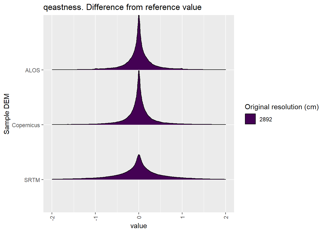
Figure 9.16: Distribution of difference between each DEM and reference for qeastness values: Algebuckina
9.1.5 qnorthness
Figure 9.17 shows rasters for qnorthness in the Algebuckina area.
Table 9.18 shows boxplots for each decile of qnorthness, allowing a comparison of values within each DEM across different ranges of qnorthness. Deciles are based on the values in the reference DEM: Outback.
Figure 9.19 shows the a distribution of values for each sample DEM and window size.
Figure 9.20 shows the distribution of differences between the reference DEM and the other DEMs.
Figure 9.17: qnorthness raster for each DEM
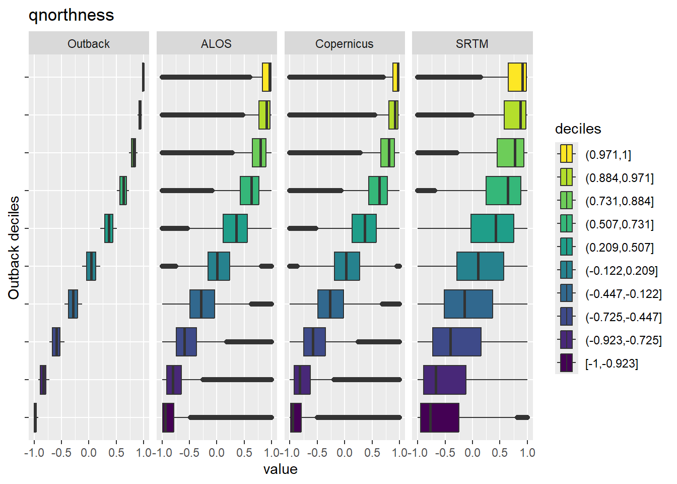
Figure 9.18: Range of values within deciles for each DEM. Deciles are taken from the reference DEM
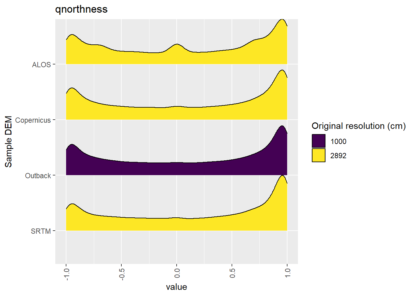
Figure 9.19: Distribution of qnorthness values in each DEM: Algebuckina
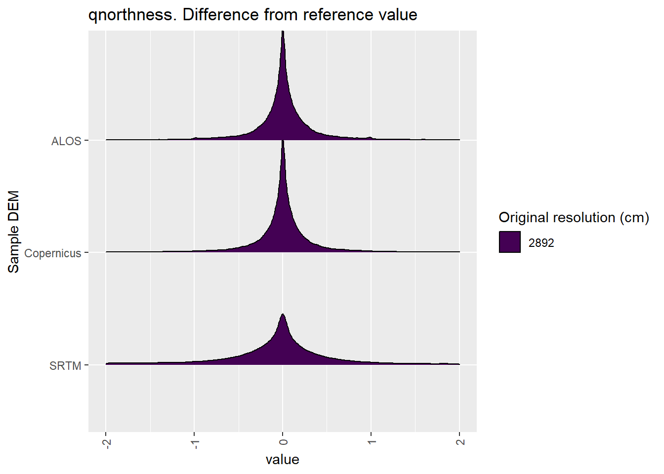
Figure 9.20: Distribution of difference between each DEM and reference for qnorthness values: Algebuckina
9.1.6 TPI
Figure 9.21 shows rasters for TPI in the Algebuckina area.
Table 9.22 shows boxplots for each decile of TPI, allowing a comparison of values within each DEM across different ranges of TPI. Deciles are based on the values in the reference DEM: Outback.
Figure 9.23 shows the a distribution of values for each sample DEM and window size.
Figure 9.24 shows the distribution of differences between the reference DEM and the other DEMs.
Figure 9.21: TPI raster for each DEM
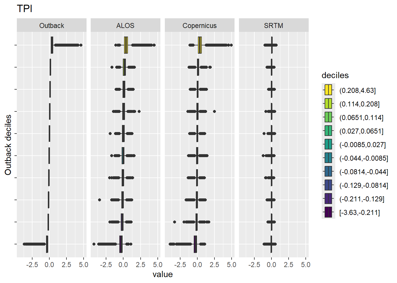
Figure 9.22: Range of values within deciles for each DEM. Deciles are taken from the reference DEM
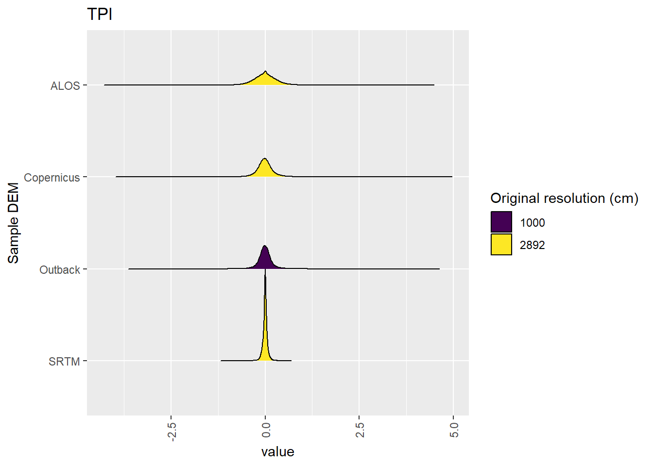
Figure 9.23: Distribution of TPI values in each DEM: Algebuckina
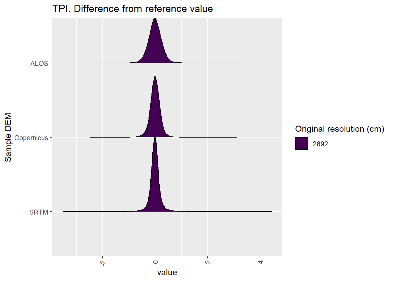
Figure 9.24: Distribution of difference between each DEM and reference for TPI values: Algebuckina
9.1.7 TRI
Figure 9.25 shows rasters for TRI in the Algebuckina area.
Table 9.26 shows boxplots for each decile of TRI, allowing a comparison of values within each DEM across different ranges of TRI. Deciles are based on the values in the reference DEM: Outback.
Figure 9.27 shows the a distribution of values for each sample DEM and window size.
Figure 9.28 shows the distribution of differences between the reference DEM and the other DEMs.
Figure 9.25: TRI raster for each DEM
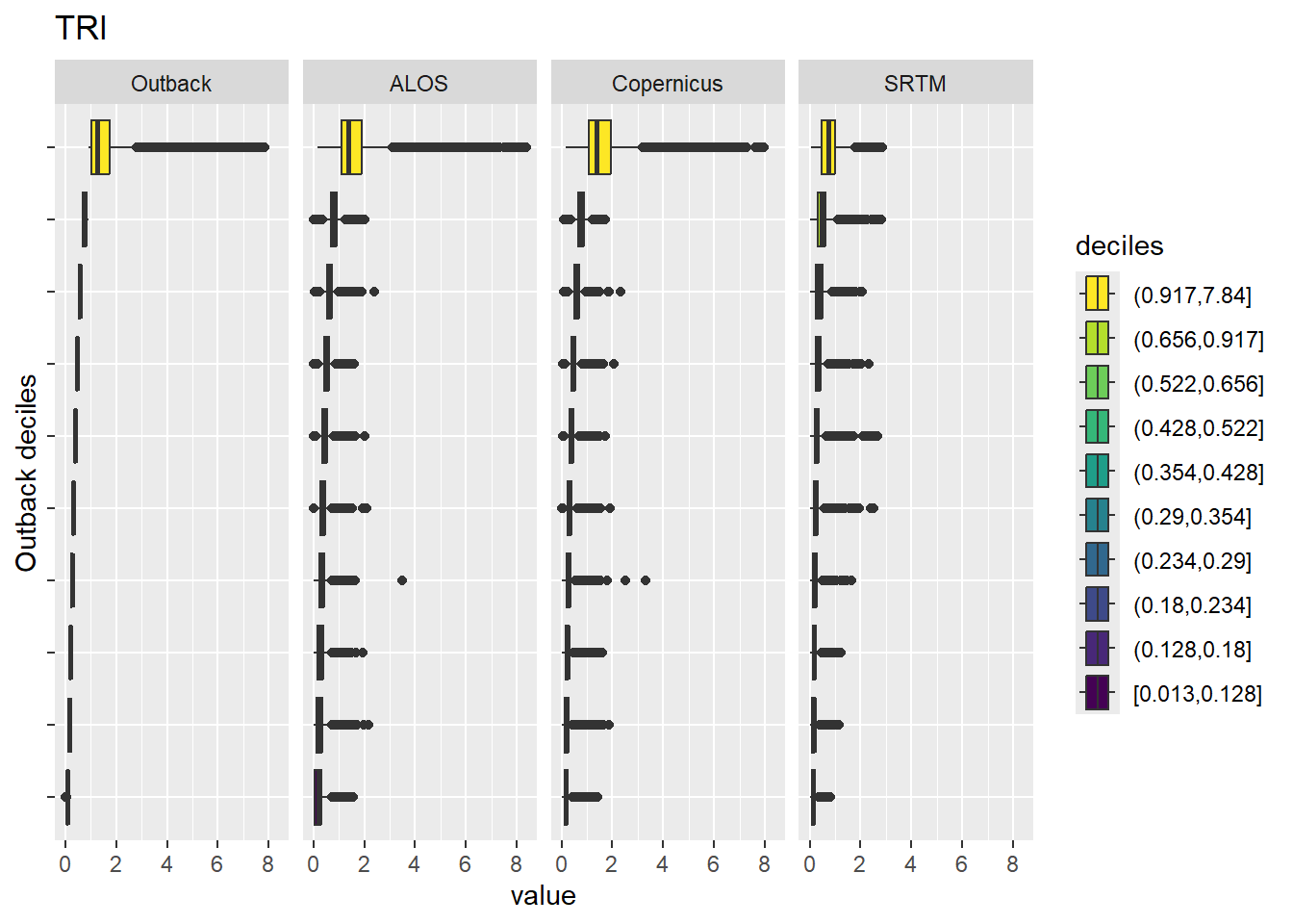
Figure 9.26: Range of values within deciles for each DEM. Deciles are taken from the reference DEM
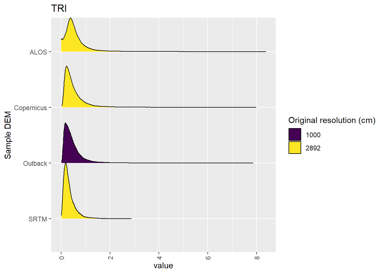
Figure 9.27: Distribution of TRI values in each DEM: Algebuckina
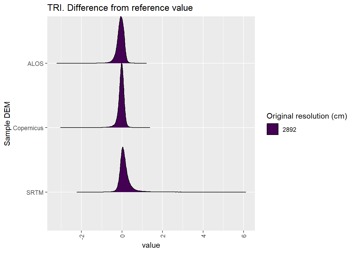
Figure 9.28: Distribution of difference between each DEM and reference for TRI values: Algebuckina
9.1.8 TRIriley
Figure 9.29 shows rasters for TRIriley in the Algebuckina area.
Table 9.30 shows boxplots for each decile of TRIriley, allowing a comparison of values within each DEM across different ranges of TRIriley. Deciles are based on the values in the reference DEM: Outback.
Figure 9.31 shows the a distribution of values for each sample DEM and window size.
Figure 9.32 shows the distribution of differences between the reference DEM and the other DEMs.
Figure 9.29: TRIriley raster for each DEM
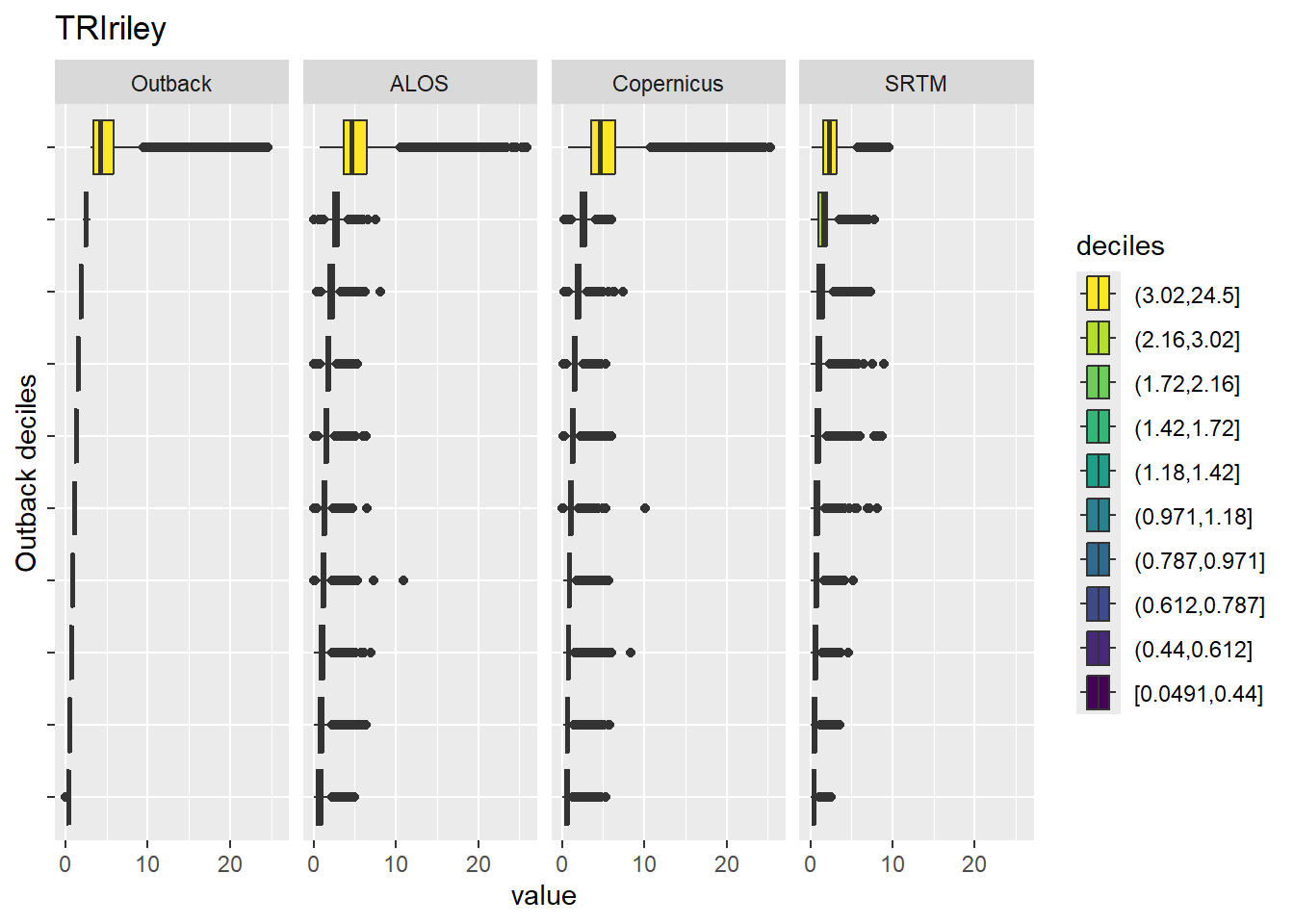
Figure 9.30: Range of values within deciles for each DEM. Deciles are taken from the reference DEM
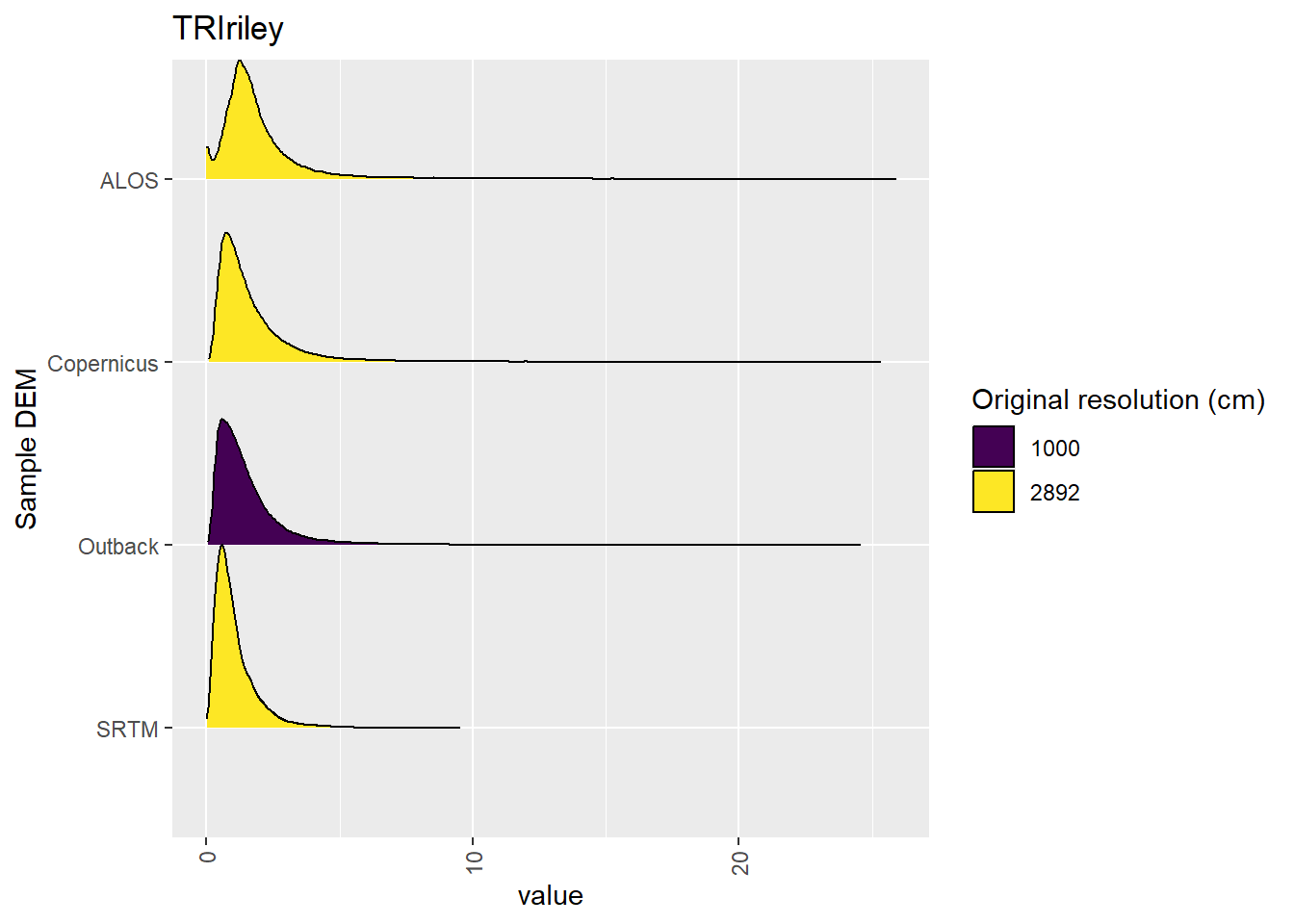
Figure 9.31: Distribution of TRIriley values in each DEM: Algebuckina
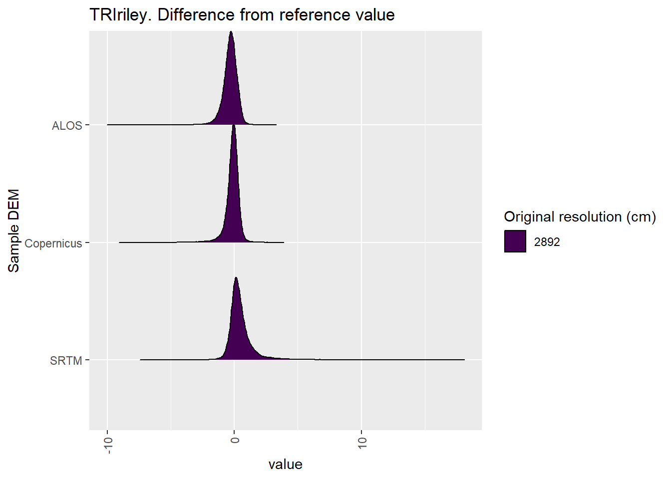
Figure 9.32: Distribution of difference between each DEM and reference for TRIriley values: Algebuckina
9.1.9 TRIrmsd
Figure 9.33 shows rasters for TRIrmsd in the Algebuckina area.
Table 9.34 shows boxplots for each decile of TRIrmsd, allowing a comparison of values within each DEM across different ranges of TRIrmsd. Deciles are based on the values in the reference DEM: Outback.
Figure 9.35 shows the a distribution of values for each sample DEM and window size.
Figure 9.36 shows the distribution of differences between the reference DEM and the other DEMs.
Figure 9.33: TRIrmsd raster for each DEM
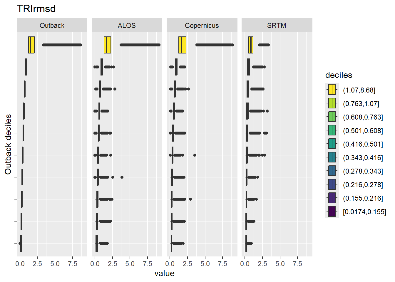
Figure 9.34: Range of values within deciles for each DEM. Deciles are taken from the reference DEM
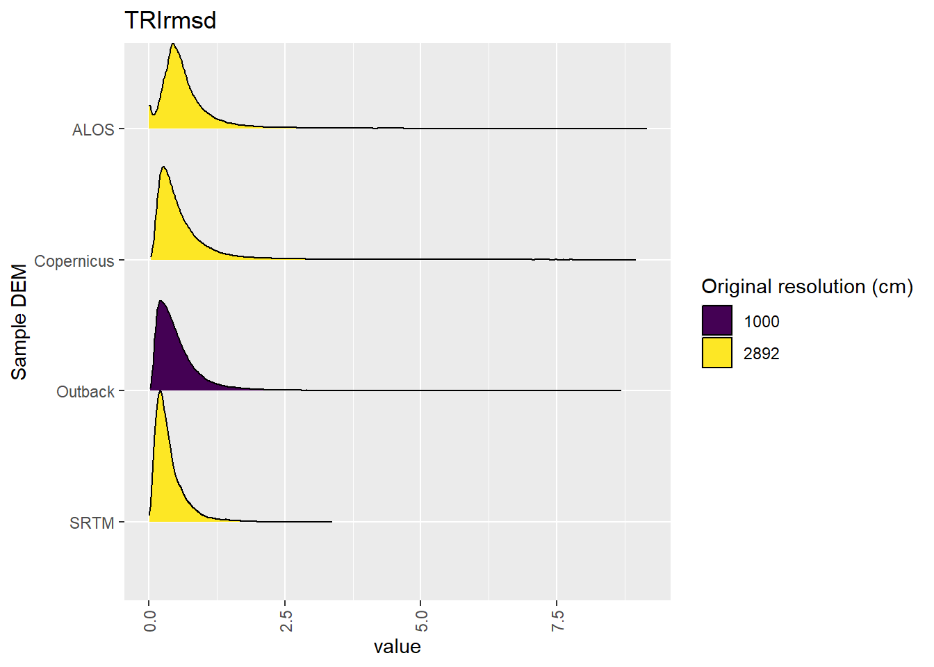
Figure 9.35: Distribution of TRIrmsd values in each DEM: Algebuckina
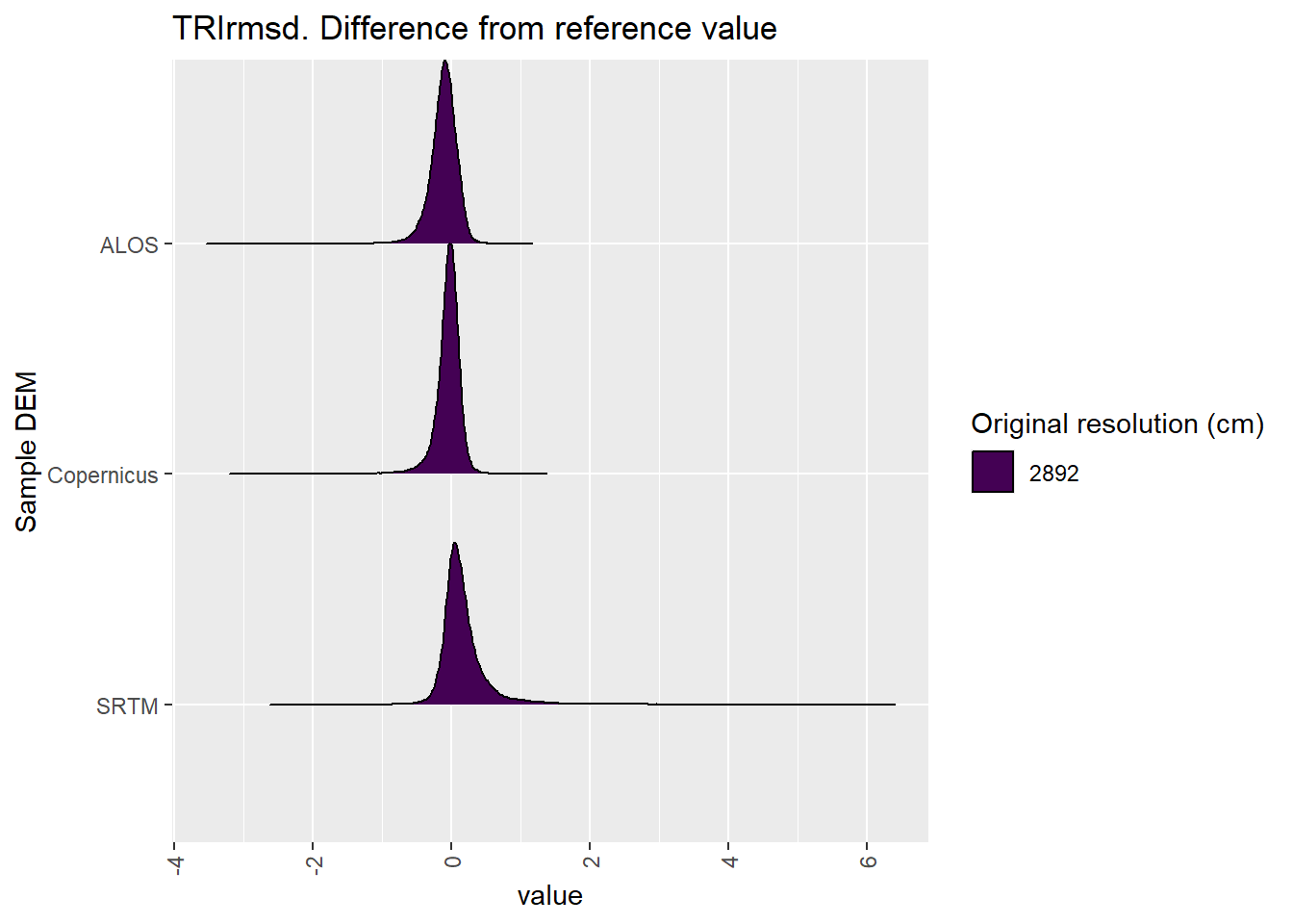
Figure 9.36: Distribution of difference between each DEM and reference for TRIrmsd values: Algebuckina
9.1.10 roughness
Figure 9.37 shows rasters for roughness in the Algebuckina area.
Table 9.38 shows boxplots for each decile of roughness, allowing a comparison of values within each DEM across different ranges of roughness. Deciles are based on the values in the reference DEM: Outback.
Figure 9.39 shows the a distribution of values for each sample DEM and window size.
Figure 9.40 shows the distribution of differences between the reference DEM and the other DEMs.
Figure 9.37: roughness raster for each DEM
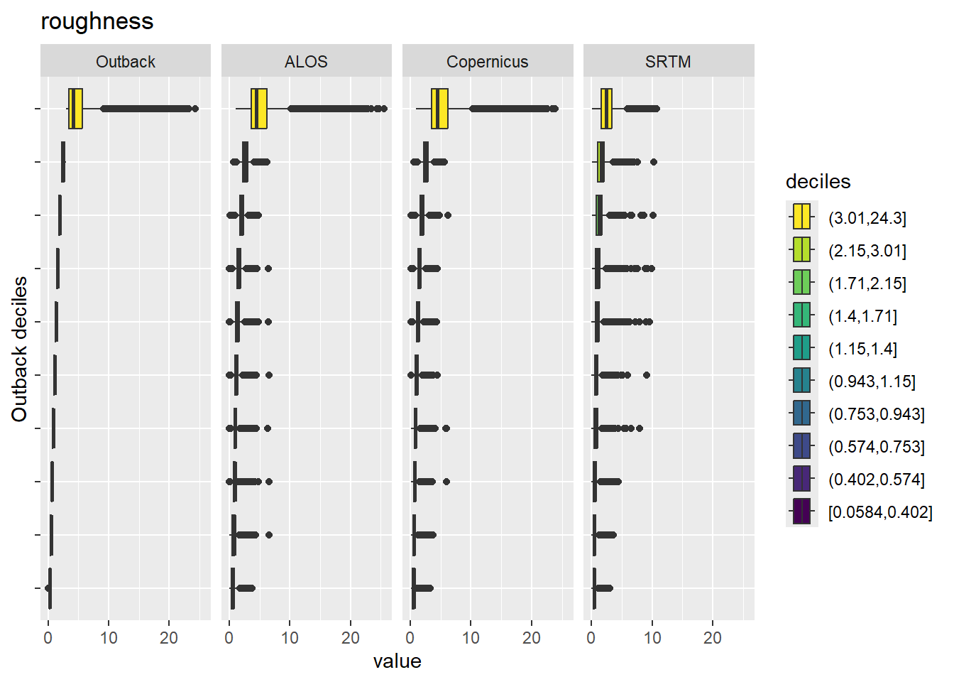
Figure 9.38: Range of values within deciles for each DEM. Deciles are taken from the reference DEM
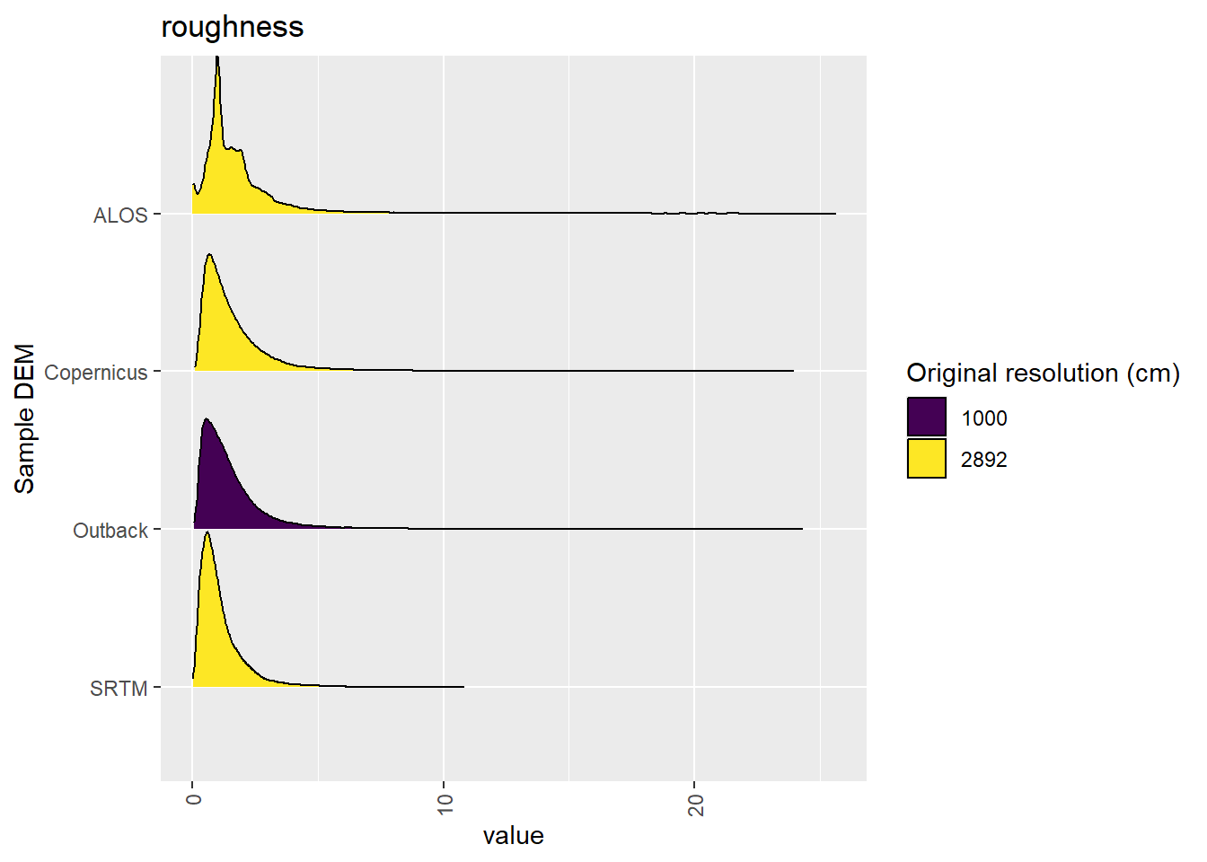
Figure 9.39: Distribution of roughness values in each DEM: Algebuckina
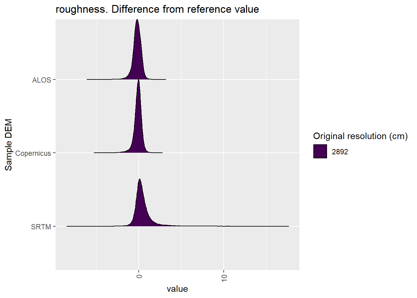
Figure 9.40: Distribution of difference between each DEM and reference for roughness values: Algebuckina
9.2 Categorical
Table 9.1 shows the proportion of each DEM classifed to each landform element (also see Figure 9.42.
Figure 9.41 shows a landscape classification for each reprojected area.
| landform | Outback | ALOS | Copernicus | SRTM |
|---|---|---|---|---|
| canyon | 0.0075 | 0.015 | 0.010 | 0.00315 |
| midslope drainage | 0.0111 | 0.019 | 0.018 | 0.00064 |
| u-shaped valley | 0.0242 | 0.028 | 0.021 | 0.02332 |
| plains | 0.8756 | 0.837 | 0.856 | 0.94676 |
| open slopes | 0.0169 | 0.020 | 0.020 | 0.00148 |
| upper slopes | 0.0453 | 0.048 | 0.047 | 0.02264 |
| midslopes ridges | 0.0103 | 0.018 | 0.016 | 0.00036 |
| mountain tops | 0.0093 | 0.015 | 0.013 | 0.00165 |
Figure 9.41: Categorical representation of Algebuckina
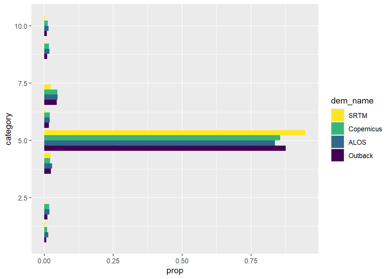
Figure 9.42: Proportion of categorised Algebuckina area in each of several classification classes